> For the complete documentation index, see [llms.txt](https://irosyadi.gitbook.io/irosyadi/llms.txt). Markdown versions of documentation pages are available by appending `.md` to page URLs; this page is available as [Markdown](https://irosyadi.gitbook.io/irosyadi/course/cs231n-summary.md).
# Standford CS231n 2017 Summary
## Table of contents
* [Standford CS231n 2017 Summary](#standford-cs231n-2017-summary)
* [Table of contents](#table-of-contents)
* [Course Info](#course-info)
* [01. Introduction to CNN for visual recognition](#01-introduction-to-cnn-for-visual-recognition)
* [02. Image classification](#02-image-classification)
* [03. Loss function and optimization](#03-loss-function-and-optimization)
* [04. Introduction to Neural network](#04-introduction-to-neural-network)
* [05. Convolutional neural networks (CNNs)](#05-convolutional-neural-networks-cnns)
* [06. Training neural networks I](#06-training-neural-networks-i)
* [07. Training neural networks II](#07-training-neural-networks-ii)
* [08. Deep learning software](#08-deep-learning-software)
* [09. CNN architectures](#09-cnn-architectures)
* [10. Recurrent Neural networks](#10-recurrent-neural-networks)
* [11. Detection and Segmentation](#11-detection-and-segmentation)
* [12. Visualizing and Understanding](#12-visualizing-and-understanding)
* [13. Generative models](#13-generative-models)
* [14. Deep reinforcement learning](#14-deep-reinforcement-learning)
* [15. Efficient Methods and Hardware for Deep Learning](#15-efficient-methods-and-hardware-for-deep-learning)
* [16. Adversarial Examples and Adversarial Training](#16-adversarial-examples-and-adversarial-training)
## Course Info
* Website:
* Lectures link:
* Full syllabus link:
* Assignments solutions:
* Number of lectures: **16**
* Course description:
* > Computer Vision has become ubiquitous in our society, with applications in search, image understanding, apps, mapping, medicine, drones, and self-driving cars. Core to many of these applications are visual recognition tasks such as image classification, localization and detection. Recent developments in neural network (aka “deep learning”) approaches have greatly advanced the performance of these state-of-the-art visual recognition systems. This course is a deep dive into details of the deep learning architectures with a focus on learning end-to-end models for these tasks, particularly image classification. During the 10-week course, students will learn to implement, train and debug their own neural networks and gain a detailed understanding of cutting-edge research in computer vision. The final assignment will involve training a multi-million parameter convolutional neural network and applying it on the largest image classification dataset (ImageNet). We will focus on teaching how to set up the problem of image recognition, the learning algorithms (e.g. backpropagation), practical engineering tricks for training and fine-tuning the networks and guide the students through hands-on assignments and a final course project. Much of the background and materials of this course will be drawn from the [ImageNet Challenge](http://image-net.org/challenges/LSVRC/2014/index).
## 01. Introduction to CNN for visual recognition
* A brief history of Computer vision starting from the late 1960s to 2017.
* Computer vision problems includes image classification, object localization, object detection, and scene understanding.
* [Imagenet](http://www.image-net.org/) is one of the biggest datasets in image classification available right now.
* Starting 2012 in the Imagenet competition, CNN (Convolutional neural networks) is always winning.
* CNN actually has been invented in 1997 by [Yann Lecun](http://ieeexplore.ieee.org/document/726791/).
## 02. Image classification
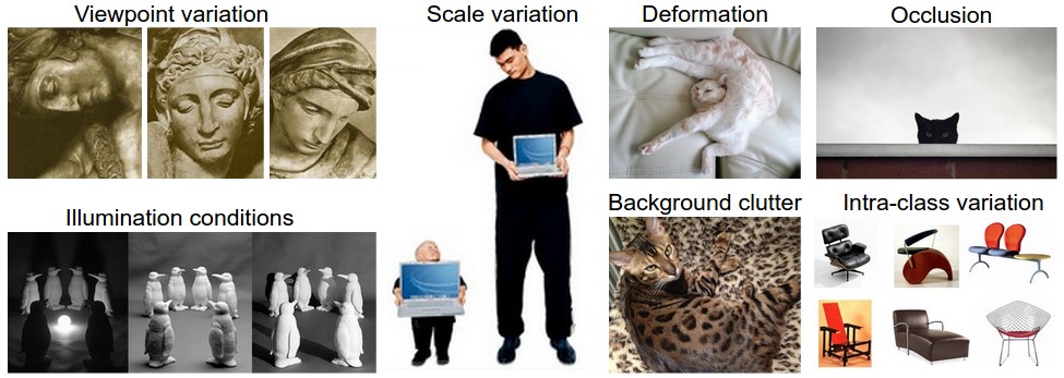
* Image classification problem has a lot of challenges like illumination and viewpoints.
* 
* An image classification algorithm can be solved with **K nearest neighborhood** (KNN) but it can poorly solve the problem. The properties of KNN are:
* Hyperparameters of KNN are: k and the distance measure
* K is the number of neighbors we are comparing to.
* Distance measures include:
* L2 distance (Euclidean distance)
* Best for non coordinate points
* L1 distance (Manhattan distance)
* Best for coordinate points
* Hyperparameters can be optimized using Cross-validation as following (In our case we are trying tp predict K):
1. Split your dataset into `f` folds.
2. Given predicted hyperparameters:
* Train your algorithm with f-1 folds and test it with the remain flood. and repeat this with every fold.
3. Choose the hyperparameters that gives the best training values (Average over all folds)
* **Linear SVM** classifier is an option for solving the image classification problem, but the curse of dimensions makes it stop improving at some point.
* **Logistic regression** is a also a solution for image classification problem, but image classification problem is non linear!
* Linear classifiers has to run the following equation: `Y = wX + b`
* shape of `w` is the same as `x` and shape of `b` is 1.
* We can add 1 to X vector and remove the bias so that: `Y = wX`
* shape of `x` is `oldX+1` and `w` is the same as `x`
* We need to know how can we get `w`'s and `b`'s that makes the classifier runs at best.
## 03. Loss function and optimization
* In the last section we talked about linear classifier but we didn't discussed how we could **train** the parameters of that model to get best `w`'s and `b`'s.
* We need a loss function to measure how good or bad our current parameters.
\*
* ```python
Loss = L[i] =(f(X[i],W),Y[i])
Loss_for_all = 1/N * Sum(Li(f(X[i],W),Y[i])) # Indicates the average
```
*
* Then we find a way to minimize the loss function given some parameters. This is called **optimization**.
* Loss function for a linear **SVM** classifier:
* `L[i] = Sum where all classes except the predicted class (max(0, s[j] - s[y[i]] + 1))`
* We call this ***the hinge loss***.
* Loss function means we are happy if the best prediction are the same as the true value other wise we give an error with 1 margin.
* Example:
* 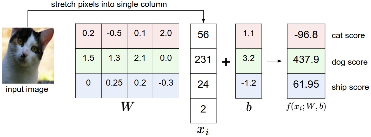
* Given this example we want to compute the loss of this image.
* `L = max (0, 437.9 - (-96.8) + 1) + max(0, 61.95 - (-96.8) + 1) = max(0, 535.7) + max(0, 159.75) = 695.45`
* Final loss is 695.45 which is big and reflects that the cat score needs to be the best over all classes as its the lowest value now. We need to minimize that loss.
* Its OK for the margin to be 1. But its a hyperparameter too.
* If your loss function gives you zero, are this value is the same value for your parameter? No there are a lot of parameters that can give you best score.
* You’ll sometimes hear about people instead using the squared hinge loss SVM (or L2-SVM). that penalizes violated margins more strongly (quadratically instead of linearly). The unsquared version is more standard, but in some datasets the squared hinge loss can work better.
* We add **regularization** for the loss function so that the discovered model don't overfit the data.
\*
* ```python
Loss = L = 1/N * Sum(Li(f(X[i],W),Y[i])) + lambda * R(W)
```
*
* Where `R` is the regularizer, and `lambda` is the regularization term.
* There are different regularizations techniques:
* | Regularizer | Equation | Comments |
| --------------------- | ----------------------------------- | ---------------------- |
| L2 | `R(W) = Sum(W^2)` | Sum all the W squared |
| L1 | `R(W) = Sum(lWl)` | Sum of all Ws with abs |
| Elastic net (L1 + L2) | `R(W) = beta * Sum(W^2) + Sum(lWl)` | |
| Dropout | | No Equation |
* Regularization prefers smaller `W`s over big `W`s.
* Regularizations is called weight decay. biases should not included in regularization.
* Softmax loss (Like linear regression but works for more than 2 classes):
* Softmax function:
\*
* ```python
A[L] = e^(score[L]) / sum(e^(score[L]), NoOfClasses)
```
*
* Sum of the vector should be 1.
* Softmax loss:
\*
* ```python
Loss = -logP(Y = y[i]|X = x[i])
```
*
* Log of the probability of the good class. We want it to be near 1 thats why we added a minus.
* Softmax loss is called cross-entropy loss.
* Consider this numerical problem when you are computing Softmax:
\*
* ```python
f = np.array([123, 456, 789]) # example with 3 classes and each having large scores
p = np.exp(f) / np.sum(np.exp(f)) # Bad: Numeric problem, potential blowup
# instead: first shift the values of f so that the highest number is 0:
f -= np.max(f) # f becomes [-666, -333, 0]
p = np.exp(f) / np.sum(np.exp(f)) # safe to do, gives the correct answer
```
*
* **Optimization**:
* How we can optimize loss functions we discussed?
* Strategy one:
* Get a random parameters and try all of them on the loss and get the best loss. But its a bad idea.
* Strategy two:
* Follow the slope.
* 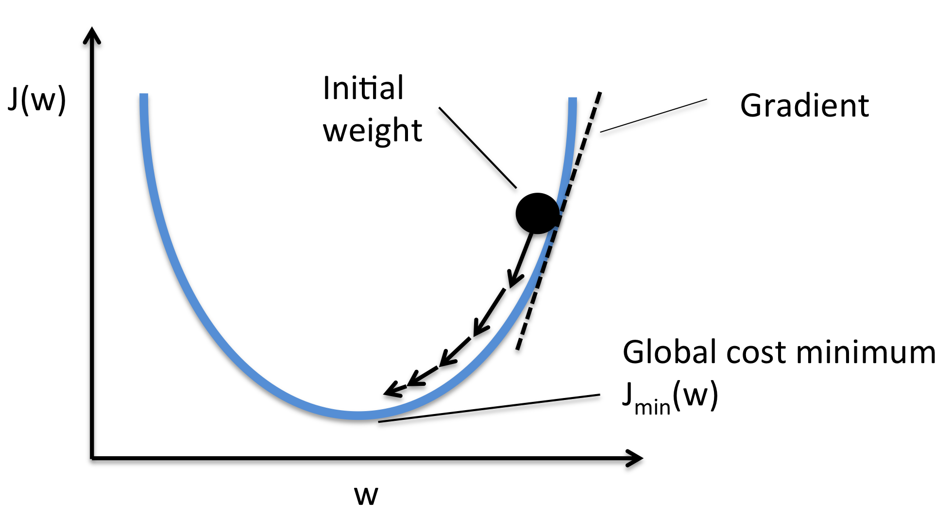
* Image [source](https://rasbt.github.io/mlxtend/user_guide/general_concepts/gradient-optimization_files/ball.png).
* Our goal is to compute the gradient of each parameter we have.
* **Numerical gradient**: Approximate, slow, easy to write. (But its useful in debugging.)
* **Analytic gradient**: Exact, Fast, Error-prone. (Always used in practice)
* After we compute the gradient of our parameters, we compute the gradient descent:
\*
* ```python
W = W - learning_rate * W_grad
```
*
* learning\_rate is so important hyper parameter you should get the best value of it first of all the hyperparameters.
* stochastic gradient descent:
* Instead of using all the date, use a mini batch of examples (32/64/128 are commonly used) for faster results.
## 04. Introduction to Neural network
* Computing the analytic gradient for arbitrary complex functions:
* What is a Computational graphs?
* Used to represent any function. with nodes.
* Using Computational graphs can easy lead us to use a technique that called back-propagation. Even with complex models like CNN and RNN.
* Back-propagation simple example:
* Suppose we have `f(x,y,z) = (x+y)z`
* Then graph can be represented this way:
*
* ```
X
\
(+)--> q ---(*)--> f
/ /
Y /
/
/
Z---------/
```
*
* We made an intermediate variable `q` to hold the values of `x+y`
* Then we have:
\*
* ```python
q = (x+y) # dq/dx = 1 , dq/dy = 1
f = qz # df/dq = z , df/dz = q
```
*
* Then:
\*
* ```python
df/dq = z
df/dz = q
df/dx = df/dq * dq/dx = z * 1 = z # Chain rule
df/dy = df/dq * dq/dy = z * 1 = z # Chain rule
```
*
* So in the Computational graphs, we call each operation `f`. For each `f` we calculate the local gradient before we go on back propagation and then we compute the gradients in respect of the loss function using the chain rule.
* In the Computational graphs you can split each operation to as simple as you want but the nodes will be a lot. if you want the nodes to be smaller be sure that you can compute the gradient of this node.
* A bigger example:
* 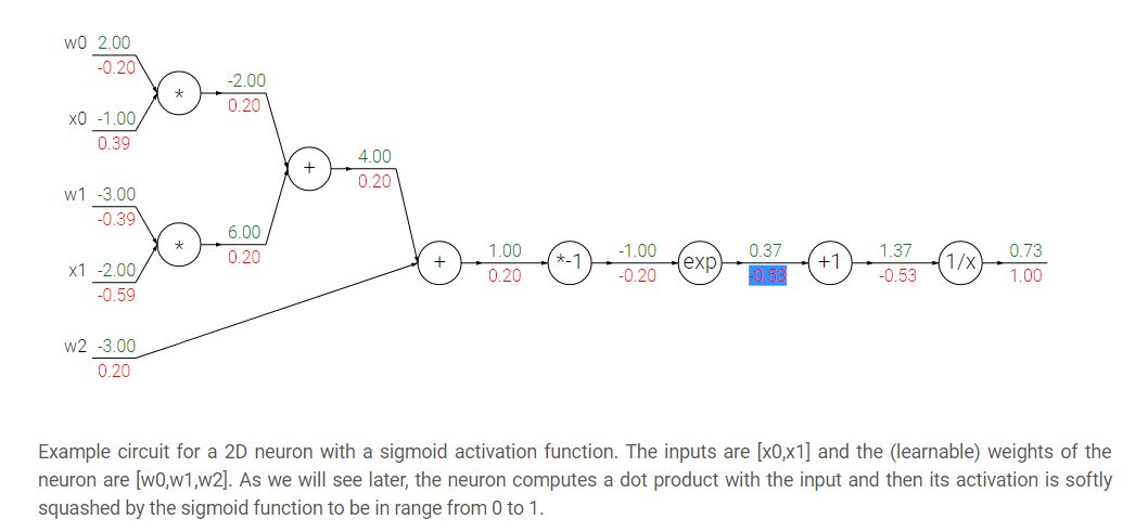
* Hint: the back propagation of two nodes going to one node from the back is by adding the two derivatives.
* Modularized implementation: forward/ backward API (example multiply code):
\*
* ```python
class MultuplyGate(object):
"""
x,y are scalars
"""
def forward(x,y):
z = x*y
self.x = x # Cache
self.y = y # Cache
# We cache x and y because we know that the derivatives contains them.
return z
def backward(dz):
dx = self.y * dz #self.y is dx
dy = self.x * dz
return [dx, dy]
```
*
* If you look at a deep learning framework you will find it follow the Modularized implementation where each class has a definition for forward and backward. For example:
* Multiplication
* Max
* Plus
* Minus
* Sigmoid
* Convolution
* So to define neural network as a function:
* (Before) Linear score function: `f = Wx`
* (Now) 2-layer neural network: `f = W2*max(0,W1*x)`
* Where max is the RELU non linear function
* (Now) 3-layer neural network: `f = W3*max(0,W2*max(0,W1*x)`
* And so on..
* Neural networks is a stack of some simple operation that forms complex operations.
## 05. Convolutional neural networks (CNNs)
* Neural networks history:
* First perceptron machine was developed by Frank Rosenblatt in 1957. It was used to recognize letters of the alphabet. Back propagation wasn't developed yet.
* Multilayer perceptron was developed in 1960 by Adaline/Madaline. Back propagation wasn't developed yet.
* Back propagation was developed in 1986 by Rumeelhart.
* There was a period which nothing new was happening with NN. Cause of the limited computing resources and data.
* In [2006](https://irosyadi.gitbook.io/irosyadi/course/www.cs.toronto.edu/~fritz/absps/netflix.pdf) Hinton released a paper that shows that we can train a deep neural network using Restricted Boltzmann machines to initialize the weights then back propagation.
* The first strong results was in 2012 by Hinton in [speech recognition](http://ieeexplore.ieee.org/document/6296526/). And the [Alexnet](https://papers.nips.cc/paper/4824-imagenet-classification-with-deep-convolutional-neural-networks.pdf) "Convolutional neural networks" that wins the image net in 2012 also by Hinton's team.
* After that NN is widely used in various applications.
* Convolutional neural networks history:
* Hubel & Wisel in 1959 to 1968 experiments on cats cortex found that there are a topographical mapping in the cortex and that the neurons has hireical organization from simple to complex.
* In 1998, Yann Lecun gives the paper [Gradient-based learning applied to document recognition](http://ieeexplore.ieee.org/document/726791/) that introduced the Convolutional neural networks. It was good for recognizing zip letters but couldn't run on a more complex examples.
* In 2012 [AlexNet](https://papers.nips.cc/paper/4824-imagenet-classification-with-deep-convolutional-neural-networks.pdf) used the same Yan Lecun architecture and won the image net challenge. The difference from 1998 that now we have a large data sets that can be used also the power of the GPUs solved a lot of performance problems.
* Starting from 2012 there are CNN that are used for various tasks (Here are some applications):
* Image classification.
* Image retrieval.
* Extracting features using a NN and then do a similarity matching.
* Object detection.
* Segmentation.
* Each pixel in an image takes a label.
* Face recognition.
* Pose recognition.
* Medical images.
* Playing Atari games with reinforcement learning.
* Galaxies classification.
* Street signs recognition.
* Image captioning.
* Deep dream.
* ConvNet architectures make the explicit assumption that the inputs are images, which allows us to encode certain properties into the architecture.
* There are a few distinct types of Layers in ConvNet (e.g. CONV/FC/RELU/POOL are by far the most popular)
* Each Layer may or may not have parameters (e.g. CONV/FC do, RELU/POOL don’t)
* Each Layer may or may not have additional hyperparameters (e.g. CONV/FC/POOL do, RELU doesn’t)
* How Convolutional neural networks works?
* A fully connected layer is a layer in which all the neurons is connected. Sometimes we call it a dense layer.
* If input shape is `(X, M)` the weighs shape for this will be `(NoOfHiddenNeurons, X)`
* Convolution layer is a layer in which we will keep the structure of the input by a filter that goes through all the image.
* We do this with dot product: `W.T*X + b`. This equation uses the broadcasting technique.
* So we need to get the values of `W` and `b`
* We usually deal with the filter (`W`) as a vector not a matrix.
* We call output of the convolution activation map. We need to have multiple activation map.
* Example if we have 6 filters, here are the shapes:
* Input image `(32,32,3)`
* filter size `(5,5,3)`
* We apply 6 filters. The depth must be three because the input map has depth of three.
* Output of Conv. `(28,28,6)`
* if one filter it will be `(28,28,1)`
* After RELU `(28,28,6)`
* Another filter `(5,5,6)`
* Output of Conv. `(24,24,10)`
* It turns out that convNets learns in the first layers the low features and then the mid-level features and then the high level features.
* After the Convnets we can have a linear classifier for a classification task.
* In Convolutional neural networks usually we have some (Conv ==> Relu)s and then we apply a pool operation to downsample the size of the activation.
* What is stride when we are doing convolution:
* While doing a conv layer we have many choices to make regarding the stride of which we will take. I will explain this by examples.
* Stride is skipping while sliding. By default its 1.
* Given a matrix with shape of `(7,7)` and a filter with shape `(3,3)`:
* If stride is `1` then the output shape will be `(5,5)` `# 2 are dropped`
* If stride is `2` then the output shape will be `(3,3)` `# 4 are dropped`
* If stride is `3` it doesn't work.
* A general formula would be `((N-F)/stride +1)`
* If stride is `1` then `O = ((7-3)/1)+1 = 4 + 1 = 5`
* If stride is `2` then `O = ((7-3)/2)+1 = 2 + 1 = 3`
* If stride is `3` then `O = ((7-3)/3)+1 = 1.33 + 1 = 2.33` `# doesn't work`
* In practice its common to zero pad the border. `# Padding from both sides.`
* Give a stride of `1` its common to pad to this equation: `(F-1)/2` where F is the filter size
* Example `F = 3` ==> Zero pad with `1`
* Example `F = 5` ==> Zero pad with `2`
* If we pad this way we call this same convolution.
* Adding zeros gives another features to the edges thats why there are different padding techniques like padding the corners not zeros but in practice zeros works!
* We do this to maintain our full size of the input. If we didn't do that the input will be shrinking too fast and we will lose a lot of data.
* Example:
* If we have input of shape `(32,32,3)` and ten filters with shape is `(5,5)` with stride `1` and pad `2`
* Output size will be `(32,32,10)` `# We maintain the size.`
* Size of parameters per filter `= 5*5*3 + 1 = 76`
* All parameters `= 76 * 10 = 76`
* Number of filters is usually common to be to the power of 2. `# To vectorize well.`
* So here are the parameters for the Conv layer:
* Number of filters K.
* Usually a power of 2.
* Spatial content size F.
* 3,5,7 ....
* The stride S.
* Usually 1 or 2 (If the stride is big there will be a downsampling but different of pooling)
* Amount of Padding
* If we want the input shape to be as the output shape, based on the F if 3 its 1, if F is 5 the 2 and so on.
* Pooling makes the representation smaller and more manageable.
* Pooling Operates over each activation map independently.
* Example of pooling is the maxpooling.
* Parameters of max pooling is the size of the filter and the stride"
* Example `2x2` with stride `2` `# Usually the two parameters are the same 2 , 2`
* Also example of pooling is average pooling.
* In this case it might be learnable.
## 06. Training neural networks I
* As a revision here are the Mini batch stochastic gradient descent algorithm steps:
* Loop:
1. Sample a batch of data.
2. Forward prop it through the graph (network) and get loss.
3. Backprop to calculate the gradients.
4. Update the parameters using the gradients.
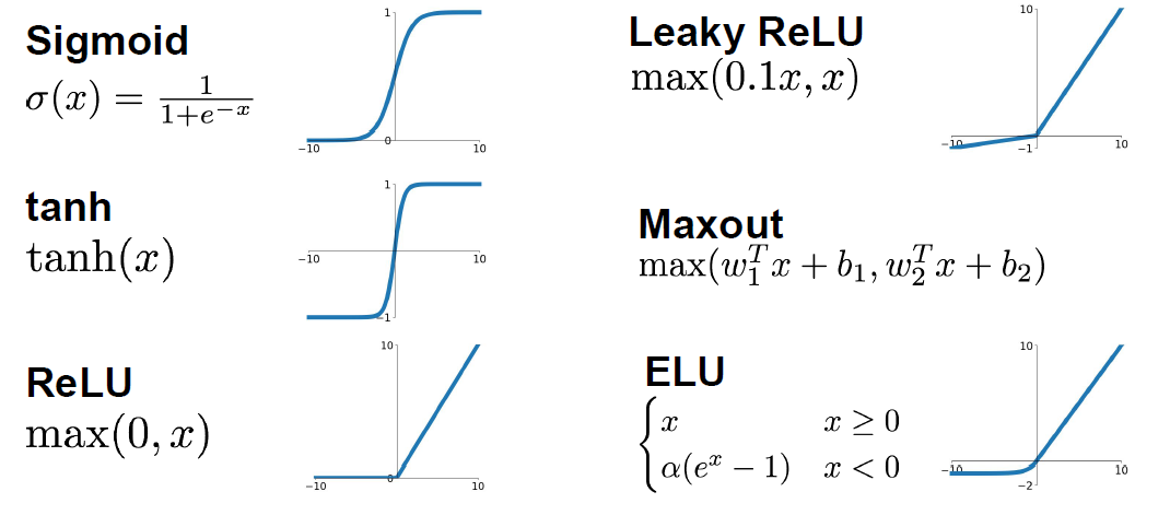
* Activation functions:
* Different choices for activation function includes Sigmoid, tanh, RELU, Leaky RELU, Maxout, and ELU.
*
```
```
* Sigmoid:
* Squashes the numbers between \[0,1]
* Used as a firing rate like human brains.
* `Sigmoid(x) = 1 / (1 + e^-x)`
* Problems with sigmoid:
* big values neurons ***kill*** the gradients.
* Gradients are in most cases near 0 (Big values/small values), that kills the updates if the graph/network are large.
* Not Zero-centered.
* Didn't produce zero-mean data.
* `exp()` is a bit compute expensive.
* just to mention. We have a more complex operations in deep learning like convolution.
* Tanh:
* Squashes the numbers between \[-1,1]
* Zero centered.
* Still big values neurons "kill" the gradients.
* `Tanh(x)` is the equation.
* Proposed by Yann Lecun in 1991.
* RELU (Rectified linear unit):
* `RELU(x) = max(0,x)`
* Doesn't kill the gradients.
* Only small values that are killed. Killed the gradient in the half
* Computationally efficient.
* Converges much faster than Sigmoid and Tanh `(6x)`
* More biologically plausible than sigmoid.
* Proposed by Alex Krizhevsky in 2012 Toronto university. (AlexNet)
* Problems:
* Not zero centered.
* If weights aren't initialized good, maybe 75% of the neurons will be dead and thats a waste computation. But its still works. This is an active area of research to optimize this.
* To solve the issue mentioned above, people might initialize all the biases by 0.01
* Leaky RELU:
* `leaky_RELU(x) = max(0.01x,x)`
* Doesn't kill the gradients from both sides.
* Computationally efficient.
* Converges much faster than Sigmoid and Tanh (6x)
* Will not die.
* PRELU is placing the 0.01 by a variable alpha which is learned as a parameter.
* Exponential linear units (ELU):
\*
* ```
ELU(x) = { x if x > 0
alpah *(exp(x) -1) if x <= 0
# alpah are a learning parameter
}
```
*
* It has all the benefits of RELU
* Closer to zero mean outputs and adds some robustness to noise.
* problems
* `exp()` is a bit compute expensive.
* Maxout activations:
* `maxout(x) = max(w1.T*x + b1, w2.T*x + b2)`
* Generalizes RELU and Leaky RELU
* Doesn't die!
* Problems:
* oubles the number of parameters per neuron
* In practice:
* Use RELU. Be careful for your learning rates.
* Try out Leaky RELU/Maxout/ELU
* Try out tanh but don't expect much.
* Don't use sigmoid!
* **Data preprocessing**:
* Normalize the data:
*
* ```python
# Zero centered data. (Calculate the mean for every input).
# On of the reasons we do this is because we need data to be between positive and negative and not all the be negative or positive.
X -= np.mean(X, axis = 1)
# Then apply the standard deviation. Hint: in images we don't do this.
X /= np.std(X, axis = 1)
```
*
* To normalize images:
* Subtract the mean image (E.g. Alexnet)
* Mean image shape is the same as the input images.
* Or Subtract per-channel mean
* Means calculate the mean for each channel of all images. Shape is 3 (3 channels)
* **Weight initialization**:
* What happened when initialize all Ws with zeros?
* All the neurons will do exactly the same thing. They will have the same gradient and they will have the same update.
* So if W's of a specific layer is equal the thing described happened
* First idea is to initialize the w's with small random numbers:
\*
* ```python
W = 0.01 * np.random.rand(D, H)
# Works OK for small networks but it makes problems with deeper networks!
```
*
* The standard deviations is going to zero in deeper networks. and the gradient will vanish sooner in deep networks.
*
* ```python
W = 1 * np.random.rand(D, H)
# Works OK for small networks but it makes problems with deeper networks!
```
*
* The network will explode with big numbers!
* ***Xavier initialization***:
\*
* ```python
W = np.random.rand(in, out) / np.sqrt(in)
```
*
* It works because we want the variance of the input to be as the variance of the output.
* But it has an issue, It breaks when you are using RELU.
* ***He initialization*** (Solution for the RELU issue):
\*
* ```python
W = np.random.rand(in, out) / np.sqrt(in/2)
```
*
* Solves the issue with RELU. Its recommended when you are using RELU
* Proper initialization is an active area of research.
* **Batch normalization**:
* is a technique to provide any layer in a Neural Network with inputs that are zero mean/unit variance.
* It speeds up the training. You want to do this a lot.
* Made by Sergey Ioffe and Christian Szegedy at 2015.
* We make a Gaussian activations in each layer. by calculating the mean and the variance.
* Usually inserted after (fully connected or Convolutional layers) and (before nonlinearity).
* Steps (For each output of a layer)\
5\. First we compute the mean and variance^2 of the batch for each feature.\
6\. We normalize by subtracting the mean and dividing by square root of (variance^2 + epsilon)
* epsilon to not divide by zero
* Then we make a scale and shift variables: `Result = gamma * normalizedX + beta`
* gamma and beta are learnable parameters.
* it basically possible to say “Hey!! I don’t want zero mean/unit variance input, give me back the raw input - it’s better for me.”
* Hey shift and scale by what you want not just the mean and variance!
* The algorithm makes each layer flexible (It chooses which distribution it wants)
* We initialize the BatchNorm Parameters to transform the input to zero mean/unit variance distributions but during training they can learn that any other distribution might be better.
* During the running of the training we need to calculate the globalMean and globalVariance for each layer by using weighted average.
* Benefits of Batch Normalization:
* Networks train faster.
* Allows higher learning rates.
* helps reduce the sensitivity to the initial starting weights.
* Makes more activation functions viable.
* Provides some regularization.
* Because we are calculating mean and variance for each batch that gives a slight regularization effect.
* In conv layers, we will have one variance and one mean per activation map.
* Batch normalization have worked best for CONV and regular deep NN, But for recurrent NN and reinforcement learning its still an active research area.
* Its challengey in reinforcement learning because the batch is small.
* **Baby sitting the learning process**
1. Preprocessing of data.
2. Choose the architecture.
3. Make a forward pass and check the loss (Disable regularization). Check if the loss is reasonable.
4. Add regularization, the loss should go up!
5. Disable the regularization again and take a small number of data and try to train the loss and reach zero loss.
* You should overfit perfectly for small datasets.
6. Take your full training data, and small regularization then try some value of learning rate.
* If loss is barely changing, then the learning rate is small.
* If you got `NAN` then your NN exploded and your learning rate is high.
* Get your learning rate range by trying the min value (That can change) and the max value that doesn't explode the network.
7. Do Hyperparameters optimization to get the best hyperparameters values.
* Hyperparameter Optimization
* Try Cross validation strategy.
* Run with a few ephocs, and try to optimize the ranges.
* Its best to optimize in log space.
* Adjust your ranges and try again.
* Its better to try random search instead of grid searches (In log space)
## 07. Training neural networks II
* **Optimization algorithms**:
* Problems with stochastic gradient descent:
* if loss quickly in one direction and slowly in another (For only two variables), you will get very slow progress along shallow dimension, jitter along steep direction. Our NN will have a lot of parameters then the problem will be more.
* Local minimum or saddle points
* If SGD went into local minimum we will stuck at this point because the gradient is zero.
* Also in saddle points the gradient will be zero so we will stuck.
* Saddle points says that at some point:
* Some gradients will get the loss up.
* Some gradients will get the loss down.
* And that happens more in high dimensional (100 million dimension for example)
* The problem of deep NN is more about saddle points than about local minimum because deep NN has high dimensions (Parameters)
* Mini batches are noisy because the gradient is not taken for the whole batch.
* **SGD + momentum**:
* Build up velocity as a running mean of gradients:
*
* ```python
# Computing weighted average. rho best is in range [0.9 - 0.99]
V[t+1] = rho * v[t] + dx
x[t+1] = x[t] - learningRate * V[t+1]
```
*
* `V[0]` is zero.
* Solves the saddle point and local minimum problems.
* It overshoots the problem and returns to it back.
* **Nestrov momentum**:
\*
* ```python
dx = compute_gradient(x)
old_v = v
v = rho * v - learning_rate * dx
x+= -rho * old_v + (1+rho) * v
```
*
* Doesn't overshoot the problem but slower than SGD + momentum
* **AdaGrad**
\*
* ```python
grad_squared = 0
while(True):
dx = compute_gradient(x)
# here is a problem, the grad_squared isn't decayed (gets so large)
grad_squared += dx * dx
x -= (learning_rate*dx) / (np.sqrt(grad_squared) + 1e-7)
```
*
* **RMSProp**
\*
* ```python
grad_squared = 0
while(True):
dx = compute_gradient(x)
#Solved ADAgra
grad_squared = decay_rate * grad_squared + (1-grad_squared) * dx * dx
x -= (learning_rate*dx) / (np.sqrt(grad_squared) + 1e-7)
```
*
* People uses this instead of AdaGrad
* **Adam**
* Calculates the momentum and RMSProp as the gradients.
* It need a Fixing bias to fix starts of gradients.
* Is the best technique so far runs best on a lot of problems.
* With `beta1 = 0.9` and `beta2 = 0.999` and `learning_rate = 1e-3` or `5e-4` is a great starting point for many models!
* **Learning decay**
* Ex. decay learning rate by half every few epochs.
* To help the learning rate not to bounce out.
* Learning decay is common with SGD+momentum but not common with Adam.
* Dont use learning decay from the start at choosing your hyperparameters. Try first and check if you need decay or not.
* All the above algorithms we have discussed is a first order optimization.
* **Second order optimization**
* Use gradient and Hessian to from quadratic approximation.
* Step to the minima of the approximation.
* What is nice about this update?
* It doesn't has a learning rate in some of the versions.
* But its unpractical for deep learning
* Has O(N^2) elements.
* Inverting takes O(N^3).
* **L-BFGS** is a version of second order optimization
* Works with batch optimization but not with mini-batches.
* In practice first use ADAM and if it didn't work try L-BFGS.
* Some says all the famous deep architectures uses **SGS + Nestrov momentum**
* **Regularization**
* So far we have talked about reducing the training error, but we care about most is how our model will handle unseen data!
* What if the gab of the error between training data and validation data are too large?
* This error is called high variance.
* **Model Ensembles**:
* Algorithm:
* Train multiple independent models of the same architecture with different initializations.
* At test time average their results.
* It can get you extra 2% performance.
* It reduces the generalization error.
* You can use some snapshots of your NN at the training ensembles them and take the results.
* Regularization solves the high variance problem. We have talked about L1, L2 Regularization.
* Some Regularization techniques are designed for only NN and can do better.
* **Drop out**:
* In each forward pass, randomly set some of the neurons to zero. Probability of dropping is a hyperparameter that are 0.5 for almost cases.
* So you will chooses some activation and makes them zero.
* It works because:
* It forces the network to have redundant representation; prevent co-adaption of features!
* If you think about this, It ensemble some of the models in the same model!
* At test time we might multiply each dropout layer by the probability of the dropout.
* Sometimes at test time we don't multiply anything and leave it as it is.
* With drop out it takes more time to train.
* **Data augmentation**:
* Another technique that makes Regularization.
* Change the data!
* For example flip the image, or rotate it.
* Example in ResNet:
* Training: Sample random crops and scales:
1. Pick random L in range \[256,480]
2. Resize training image, short side = L
3. Sample random 224x244 patch.
* Testing: average a fixed set of crops\
4\. Resize image at 5 scales: {224, 256, 384, 480, 640}\
5\. For each size, use 10 224x224 crops: 4 corners + center + flips
* Apply Color jitter or PCA
* Translation, rotation, stretching.
* Drop connect
* Like drop out idea it makes a regularization.
* Instead of dropping the activation, we randomly zeroing the weights.
* Fractional Max Pooling
* Cool regularization idea. Not commonly used.
* Randomize the regions in which we pool.
* Stochastic depth
* New idea.
* Eliminate layers, instead on neurons.
* Has the similar effect of drop out but its a new idea.
* **Transfer learning**:
* Some times your data is overfitted by your model because the data is small not because of regularization.
* You need a lot of data if you want to train/use CNNs.
* Steps of transfer learning
1. Train on a big dataset that has common features with your dataset. Called pretraining.
2. Freeze the layers except the last layer and feed your small dataset to learn only the last layer.
3. Not only the last layer maybe trained again, you can fine tune any number of layers you want based on the number of data you have
* Guide to use transfer learning:
* | | Very Similar dataset | very different dataset |
| ----------------------- | ---------------------------------- | --------------------------------------------------------------- |
| **very little dataset** | Use Linear classifier on top layer | You're in trouble.. Try linear classifier from different stages |
| **quite a lot of data** | Finetune a few layers | Finetune a large layers |
* Transfer learning is the normal not an exception.
## 08. Deep learning software
* This section changes a lot every year in CS231n due to rabid changes in the deep learning softwares.
* CPU vs GPU
* GPU The graphics card was developed to render graphics to play games or make 3D media,. etc.
* NVIDIA vs AMD
* Deep learning choose NVIDIA over AMD GPU because NVIDIA is pushing research forward deep learning also makes it architecture more suitable for deep learning.
* CPU has fewer cores but each core is much faster and much more capable; great at sequential tasks. While GPUs has more cores but each core is much slower "dumber"; great for parallel tasks.
* GPU cores needs to work together. and has its own memory.
* Matrix multiplication is from the operations that are suited for GPUs. It has MxN independent operations that can be done on parallel.
* Convolution operation also can be paralyzed because it has independent operations.
* Programming GPUs frameworks:
* **CUDA** (NVIDIA only)
* Write c-like code that runs directly on the GPU.
* Its hard to build a good optimized code that runs on GPU. Thats why they provided high level APIs.
* Higher level APIs: cuBLAS, cuDNN, etc
* **CuDNN** has implemented back prop. , convolution, recurrent and a lot more for you!
* In practice you won't write a parallel code. You will use the code implemented and optimized by others!
* **OpenCl**
* Similar to CUDA, but runs on any GPU.
* Usually Slower .
* Haven't much support yet from all deep learning softwares.
* There are a lot of courses for learning parallel programming.
* If you aren't careful, training can bottleneck on reading dara and transferring to GPU. So the solutions are:
* Read all the data into RAM. # If possible
* Use SSD instead of HDD
* Use multiple CPU threads to prefetch data!
* While the GPU are computing, a CPU thread will fetch the data for you.
* A lot of frameworks implemented that for you because its a little bit painful!
* **Deep learning Frameworks**
* Its super fast moving!
* Currently available frameworks:
* Tensorflow (Google)
* Caffe (UC Berkeley)
* Caffe2 (Facebook)
* Torch (NYU / Facebook)
* PyTorch (Facebook)
* Theano (U monteral)
* Paddle (Baidu)
* CNTK (Microsoft)
* MXNet (Amazon)
* The instructor thinks that you should focus on Tensorflow and PyTorch.
* The point of deep learning frameworks:
* Easily build big computational graphs.
* Easily compute gradients in computational graphs.
* Run it efficiently on GPU (cuDNN - cuBLAS)
* Numpy doesn't run on GPU.
* Most of the frameworks tries to be like NUMPY in the forward pass and then they compute the gradients for you.
* **Tensorflow (Google)**
* Code are two parts:
1. Define computational graph.
2. Run the graph and reuse it many times.
* Tensorflow uses a static graph architecture.
* Tensorflow variables live in the graph. while the placeholders are feed each run.
* Global initializer function initializes the variables that lives in the graph.
* Use predefined optimizers and losses.
* You can make a full layers with layers.dense function.
* **Keras** (High level wrapper):
* Keras is a layer on top pf Tensorflow, makes common things easy to do.
* So popular!
* Trains a full deep NN in a few lines of codes.
* There are a lot high level wrappers:
* Keras
* TFLearn
* TensorLayer
* tf.layers `#Ships with tensorflow`
* tf-Slim `#Ships with tensorflow`
* tf.contrib.learn `#Ships with tensorflow`
* Sonnet `# New from deep mind`
* Tensorflow has pretrained models that you can use while you are using transfer learning.
* Tensorboard adds logging to record loss, stats. Run server and get pretty graphs!
* It has distributed code if you want to split your graph on some nodes.
* Tensorflow is actually inspired from Theano. It has the same inspirations and structure.
* **PyTorch (Facebook)**
* Has three layers of abstraction:
* Tensor: `ndarray` but runs on GPU `#Like numpy arrays in tensorflow`
* Variable: Node in a computational graphs; stores data and gradient `#Like Tensor, Variable, Placeholders`
* Module: A NN layer; may store state or learnable weights`#Like tf.layers in tensorflow`
* In PyTorch the graphs runs in the same loop you are executing which makes it easier for debugging. This is called a dynamic graph.
* In PyTorch you can define your own autograd functions by writing forward and backward for tensors. Most of the times it will implemented for you.
* Torch.nn is a high level api like keras in tensorflow. You can create the models and go on and on.
* You can define your own nn module!
* Also Pytorch contains optimizers like tensorflow.
* It contains a data loader that wraps a Dataset and provides minbatches, shuffling and multithreading.
* PyTorch contains the best and super easy to use pretrained models
* PyTorch contains Visdom that are like tensorboard. but Tensorboard seems to be more powerful.
* PyTorch is new and still evolving compared to Torch. Its still in beta state.
* PyTorch is best for research.
* Tensorflow builds the graph once, then run them many times (Called static graph)
* In each PyTorch iteration we build a new graph (Called dynamic graph)
* **Static vs dynamic graphs**:
* Optimization:
* With static graphs, framework can optimize the graph for you before it runs.
* Serialization
* **Static**: Once graph is built, can serialize it and run it without the code that built the graph. Ex use the graph in c++
* **Dynamic**: Always need to keep the code around.
* Conditional
* Is easier in dynamic graphs. And more complicated in static graphs.
* Loops:
* Is easier in dynamic graphs. And more complicated in static graphs.
* Tensorflow fold make dynamic graphs easier in Tensorflow through dynamic batching.
* Dynamic graph applications include: recurrent networks and recursive networks.
* Caffe2 uses static graphs and can train model in python also works on IOS and Android
* Tensorflow/Caffe2 are used a lot in production especially on mobile.
## 09. CNN architectures
* This section talks about the famous CNN architectures. Focuses on CNN architectures that won [ImageNet](https://irosyadi.gitbook.io/irosyadi/course/www.image-net.org) competition since 2012.
* 
* These architectures includes: [AlexNet](https://papers.nips.cc/paper/4824-imagenet-classification-with-deep-convolutional-neural-networks.pdf), [VGG](https://arxiv.org/abs/1409.1556), [GoogLeNet](https://research.google.com/pubs/pub43022.html), and [ResNet](https://arxiv.org/abs/1512.03385).
* Also we will discuss some interesting architectures as we go.
* The first ConvNet that was made was [LeNet-5](http://ieeexplore.ieee.org/document/726791/) architectures are:by Yann Lecun at 1998.
* Architecture are: `CONV-POOL-CONV-POOL-FC-FC-FC`
* 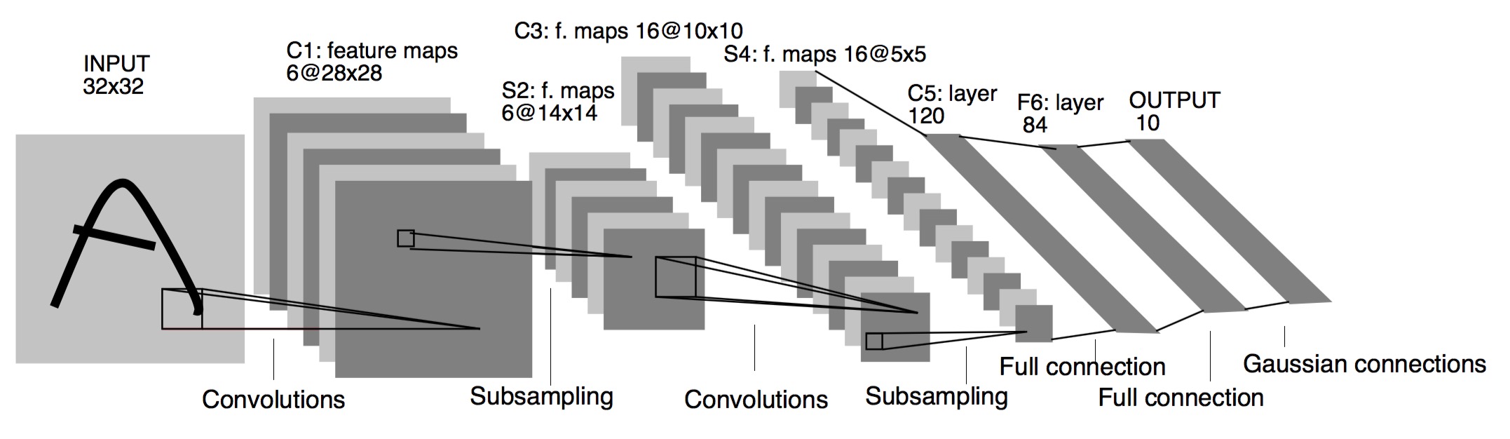
* Each conv filters was `5x5` applied at stride 1
* Each pool was `2x2` applied at stride `2`
* It was useful in Digit recognition.
* In particular the insight that image features are distributed across the entire image, and convolutions with learnable parameters are an effective way to extract similar features at multiple location with few parameters.
* It contains exactly **5** layers
* In [2010](https://arxiv.org/abs/1003.0358) Dan Claudiu Ciresan and Jurgen Schmidhuber published one of the very fist implementations of GPU Neural nets. This implementation had both forward and backward implemented on a a NVIDIA GTX 280 graphic processor of an up to 9 layers neural network.
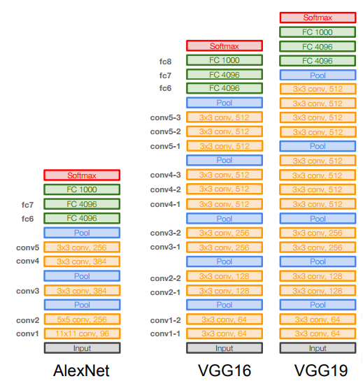
* [**AlexNet**](https://papers.nips.cc/paper/4824-imagenet-classification-with-deep-convolutional-neural-networks.pdf) (2012):
* ConvNet that started the evolution and wins the ImageNet at 2012.
* Architecture are: `CONV1-MAXPOOL1-NORM1-CONV2-MAXPOOL2-NORM2-CONV3-CONV4-CONV5-MAXPOOL3-FC6-FC7-FC8`
* Contains exactly **8** layers the first 5 are Convolutional and the last 3 are fully connected layers.
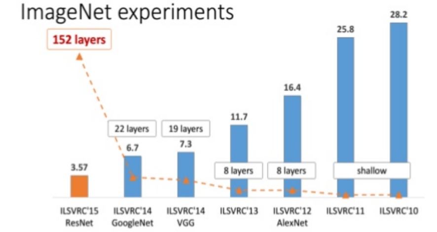
* AlexNet accuracy error was `16.4%`
* For example if the input is 227 x 227 x3 then these are the shapes of the of the outputs at each layer:
* CONV1 (96 11 x 11 filters at stride 4, pad 0)
* Output shape `(55,55,96)`, Number of weights are `(11*11*3*96)+96 = 34944`
* MAXPOOL1 (3 x 3 filters applied at stride 2)
* Output shape `(27,27,96)`, No Weights
* NORM1
* Output shape `(27,27,96)`, We don't do this any more
* CONV2 (256 5 x 5 filters at stride 1, pad 2)
* MAXPOOL2 (3 x 3 filters at stride 2)
* NORM2
* CONV3 (384 3 x 3 filters ar stride 1, pad 1)
* CONV4 (384 3 x 3 filters ar stride 1, pad 1)
* CONV5 (256 3 x 3 filters ar stride 1, pad 1)
* MAXPOOL3 (3 x 3 filters at stride 2)
* Output shape `(6,6,256)`
* FC6 (4096)
* FC7 (4096)
* FC8 (1000 neurons for class score)
* Some other details:
* First use of RELU.
* Norm layers but not used any more.
* heavy data augmentation
* Dropout `0.5`
* batch size `128`
* SGD momentum `0.9`
* Learning rate `1e-2` reduce by 10 at some iterations
* 7 CNN ensembles!
* AlexNet was trained on GTX 580 GPU with only 3 GB which wasn't enough to train in one machine so they have spread the feature maps in half. The first AlexNet was distributed!
* Its still used in transfer learning in a lot of tasks.
* Total number of parameters are `60 million`
* [**ZFNet**](https://arxiv.org/abs/1311.2901) (2013)
* Won in 2013 with error 11.7%
* It has the same general structure but they changed a little in hyperparameters to get the best output.
* Also contains **8** layers.
* AlexNet but:
* `CONV1`: change from (11 x 11 stride 4) to (7 x 7 stride 2)
* `CONV3,4,5`: instead of 384, 384, 256 filters use 512, 1024, 512
* [OverFeat](https://arxiv.org/abs/1312.6229) (2013)
* Won the localization in imageNet in 2013
* We show how a multiscale and sliding window approach can be efficiently implemented within a ConvNet. We also introduce a novel deep learning approach to localization by learning to predict object boundaries.
* [**VGGNet**](https://arxiv.org/pdf/1409.1556) (2014) (Oxford)
* Deeper network with more layers.
* Contains 19 layers.
* Won on 2014 with GoogleNet with error 7.3%
* Smaller filters with deeper layers.
* The great advantage of VGG was the insight that multiple 3 × 3 convolution in sequence can emulate the effect of larger receptive fields, for examples 5 × 5 and 7 × 7.
* Used the simple 3 x 3 Conv all through the network.
* 3 (3 x 3) filters has the same effect as 7 x 7
* 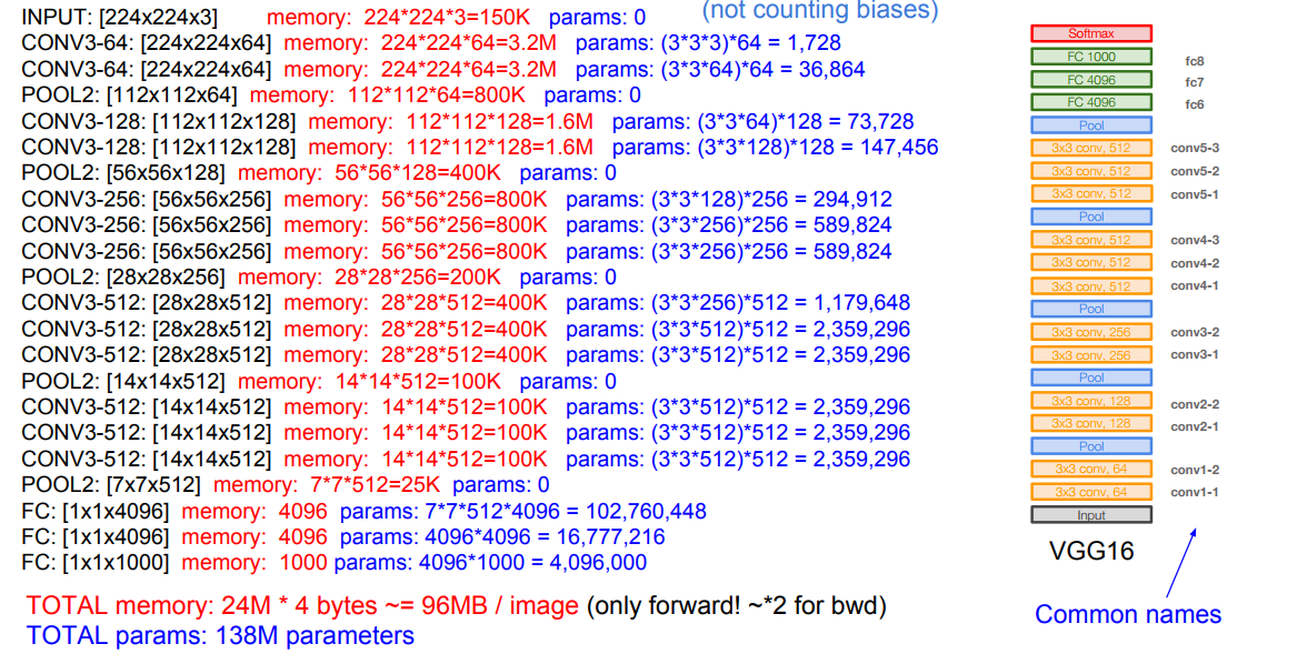
* The Architecture contains several CONV layers then POOL layer over 5 times and then the full connected layers.
* It has a total memory of 96MB per image for only forward propagation!
* Most memory are in the earlier layers
* Total number of parameters are 138 million
* Most of the parameters are in the fully connected layers
* Has a similar details in training like AlexNet. Like using momentum and dropout.
* VGG19 are an upgrade for VGG16 that are slightly better but with more memory
* 
* [**GoogleNet**](https://research.google.com/pubs/pub43022.html) (2014)
* Deeper network with more layers.
* Contains 22 layers.
* It has Efficient **Inception** module.
* Only 5 million parameters! 12x less than AlexNet
* Won on 2014 with VGGNet with error 6.7%
* Inception module:
* Design a good local network topology (network within a network (NiN)) and then stack these modules on top of each other.
* It consists of:
* Apply parallel filter operations on the input from previous layer
* Multiple convs of sizes (1 x 1, 3 x 3, 5 x 5)
* Adds padding to maintain the sizes.
* Pooling operation. (Max Pooling)
* Adds padding to maintain the sizes.
* Concatenate all filter outputs together depth-wise.
* For example:
* Input for inception module is 28 x 28 x 256
* Then the parallel filters applied:
* (1 x 1), 128 filter `# output shape (28,28,128)`
* (3 x 3), 192 filter `# output shape (28,28,192)`
* (5 x 5), 96 filter `# output shape (28,28,96)`
* (3 x 3) Max pooling `# output shape (28,28,256)`
* After concatenation this will be `(28,28,672)`
* By this design -We call Naiveit has a big computation complexity.
* The last example will make:
* \[1 x 1 conv, 128] ==> 28 \* 28 \* 128 \* 1 \* 1 \* 256 = 25 Million approx
* \[3 x 3 conv, 192] ==> 28 \* 28 \* 192 \*3 \*3 \* 256 = 346 Million approx
* \[5 x 5 conv, 96] ==> 28 \* 28 \* 96 \* 5 \* 5 \* 256 = 482 Million approx
* In total around 854 Million operation!
* Solution: **bottleneck** layers that use 1x1 convolutions to reduce feature depth.
* Inspired from NiN ([Network in network](https://arxiv.org/abs/1312.4400))
* 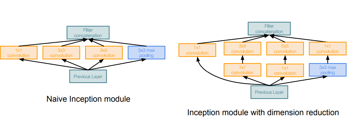
* The bottleneck solution will make a total operations of 358M on this example which is good compared with the naive implementation.
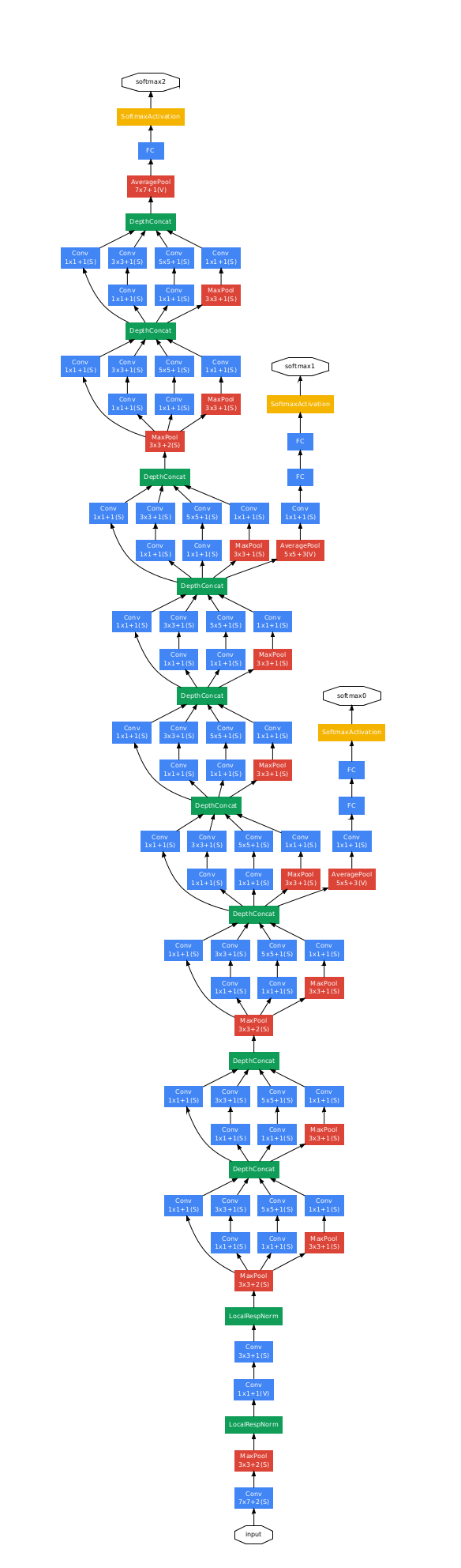
* So GoogleNet stacks this Inception module multiple times to get a full architecture of a network that can solve a problem without the Fully connected layers.
* Just to mention, it uses an average pooling layer at the end before the classification step.
* Full architecture:
* 
* In February 2015 Batch-normalized Inception was introduced as Inception V2. Batch-normalization computes the mean and standard-deviation of all feature maps at the output of a layer, and normalizes their responses with these values.
* In December [2015](https://arxiv.org/abs/1512.00567) they introduced a paper "Rethinking the Inception Architecture for Computer Vision" which explains the older inception models well also introducing a new version V3.
* The first GoogleNet and VGG was before batch normalization invented so they had some hacks to train the NN and converge well.
* [**ResNet**](https://arxiv.org/abs/1512.03385) (2015) (Microsoft Research)
* 152-layer model for ImageNet. Winner by 3.57% which is more than human level error.
* This is also the very first time that a network of > hundred, even 1000 layers was trained.
* Swept all classification and detection competitions in ILSVRC’15 and COCO’15!
* What happens when we continue stacking deeper layers on a “plain” Convolutional neural network?
* The deeper model performs worse, but it’s not caused by overfitting!
* The learning stops performs well somehow because deeper NN are harder to optimize!
* The deeper model should be able to perform at least as well as the shallower model.
* A solution by construction is copying the learned layers from the shallower model and setting additional layers to identity mapping.
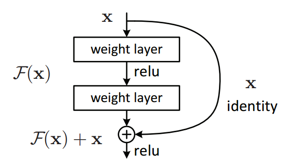
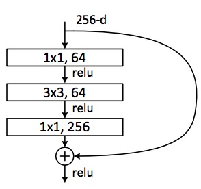
* Residual block:
* Microsoft came with the Residual block which has this architecture:
* 
*
* ```python
# Instead of us trying To learn a new representation, We learn only Residual
Y = (W2* RELU(W1x+b1) + b2) + X
```
*
* Say you have a network till a depth of N layers. You only want to add a new layer if you get something extra out of adding that layer.
* One way to ensure this new (N+1)th layer learns something new about your network is to also provide the input(x) without any transformation to the output of the (N+1)th layer. This essentially drives the new layer to learn something different from what the input has already encoded.
* The other advantage is such connections help in handling the Vanishing gradient problem in very deep networks.
* With the Residual block we can now have a deep NN of any depth without the fearing that we can't optimize the network.
* ResNet with a large number of layers started to use a bottleneck layer similar to the Inception bottleneck to reduce the dimensions.
* 
* **Full ResNet architecture**:
* Stack residual blocks.
* 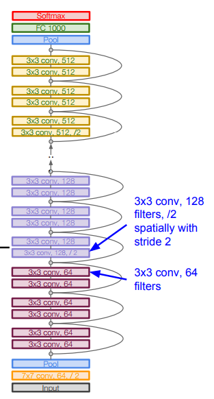
* Every residual block has two 3 x 3 conv layers.
* Additional conv layer at the beginning.
* No FC layers at the end (only FC 1000 to output classes)
* Periodically, double number of filters and downsample spatially using stride 2 (/2 in each dimension)
* Training ResNet in practice:
* Batch Normalization after every CONV layer.
* Xavier/2 initialization from He et al.
* SGD + Momentum (`0.9`)
* Learning rate: 0.1, divided by 10 when validation error plateaus
* Mini-batch size `256`
* Weight decay of `1e-5`
* No dropout used.
* [Inception-v4](https://arxiv.org/abs/1602.07261): Resnet + Inception and was founded in 2016.
* The complexity comparing over all the architectures:
* 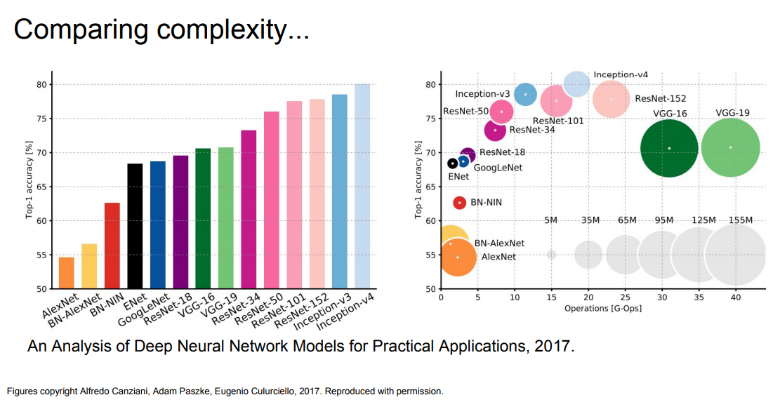
* VGG: Highest memory, most operations.
* GoogLeNet: most efficient.
* **ResNets Improvements**:
* ([2016](https://arxiv.org/abs/1603.05027)) Identity Mappings in Deep Residual Networks
* From the creators of ResNet.
* Gives better performance.
* ([2016](https://arxiv.org/abs/1605.07146)) Wide Residual Networks
* Argues that residuals are the important factor, not depth
* 50-layer wide ResNet outperforms 152-layer original ResNet
* Increasing width instead of depth more computationally efficient (parallelizable)
* ([2016](https://arxiv.org/abs/1603.09382)) Deep Networks with Stochastic Depth
* Motivation: reduce vanishing gradients and training time through short networks during training.
* Randomly drop a subset of layers during each training pass
* Use full deep network at test time.
* **Beyond ResNets**:
* ([2017](https://arxiv.org/abs/1605.07648)) FractalNet: Ultra-Deep Neural Networks without Residuals
* Argues that key is transitioning effectively from shallow to deep and residual representations are not necessary.
* Trained with dropping out sub-paths
* Full network at test time.
* ([2017](https://arxiv.org/abs/1608.06993)) Densely Connected Convolutional Networks
* ([2017](https://arxiv.org/abs/1602.07360)) SqueezeNet: AlexNet-level Accuracy With 50x Fewer Parameters and <0.5Mb Model Size
* Good for production.
* It is a re-hash of many concepts from ResNet and Inception, and show that after all, a better design of architecture will deliver small network sizes and parameters without needing complex compression algorithms.
* Conclusion:
* ResNet current best default.
* Trend towards extremely deep networks
* In the last couple of years, some models all using the shortcuts like "ResNet" to eaisly flow the gradients.
## 10. Recurrent Neural networks
* Vanilla Neural Networks "Feed neural networks", input of fixed size goes through some hidden units and then go to output. We call it a one to one network.
* Recurrent Neural Networks RNN Models:
* 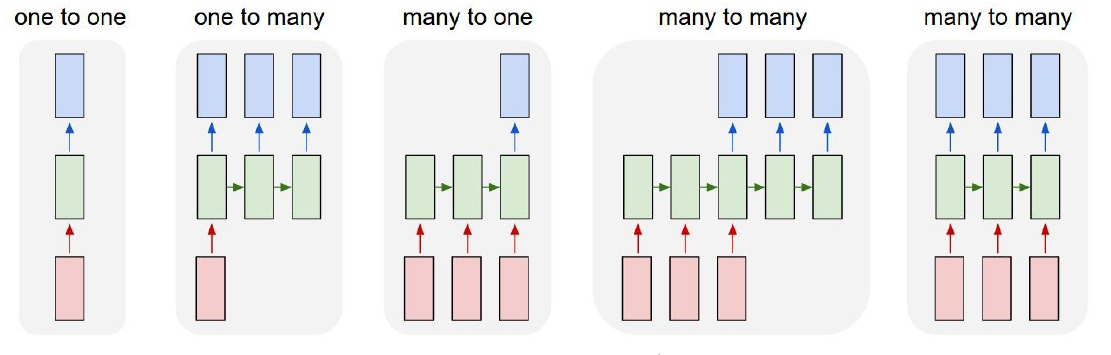
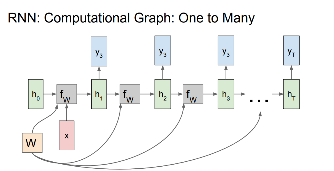
* One to many
* Example: Image Captioning
* image ==> sequence of words
* Many to One
* Example: Sentiment Classification
* sequence of words ==> sentiment
* Many to many
* Example: Machine Translation
* seq of words in one language ==> seq of words in another language
* Example: Video classification on frame level
* RNNs can also work for Non-Sequence Data (One to One problems)
* It worked in Digit classification through taking a series of “glimpses”
* “[Multiple Object Recognition with Visual Attention](https://arxiv.org/abs/1412.7755)”, ICLR 2015.
* It worked on generating images one piece at a time
* i.e generating a [captcha](http://ieeexplore.ieee.org/document/7966808/)
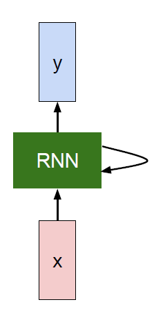
* So what is a recurrent neural network?
* Recurrent core cell that take an input x and that cell has an internal state that are updated each time it reads an input.
*
```
```
* The RNN block should return a vector.
* We can process a sequence of vectors x by applying a recurrence formula at every time step:
\*
* ```python
h[t] = fw (h[t-1], x[t]) # Where fw is some function with parameters W
```
*
* The same function and the same set of parameters are used at every time step.
* (Vanilla) Recurrent Neural Network:
\*
* ```
h[t] = tanh (W[h,h]*h[t-1] + W[x,h]*x[t]) # Then we save h[t]
y[t] = W[h,y]*h[t]
```
*
* This is the simplest example of a RNN.
* RNN works on a sequence of related data.
* Recurrent NN Computational graph:
* 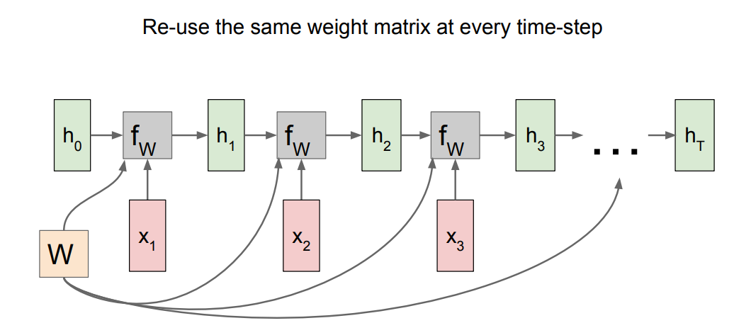
* `h0` are initialized to zero.
* Gradient of `W` is the sum of all the `W` gradients that has been calculated!
* A many to many graph:
* 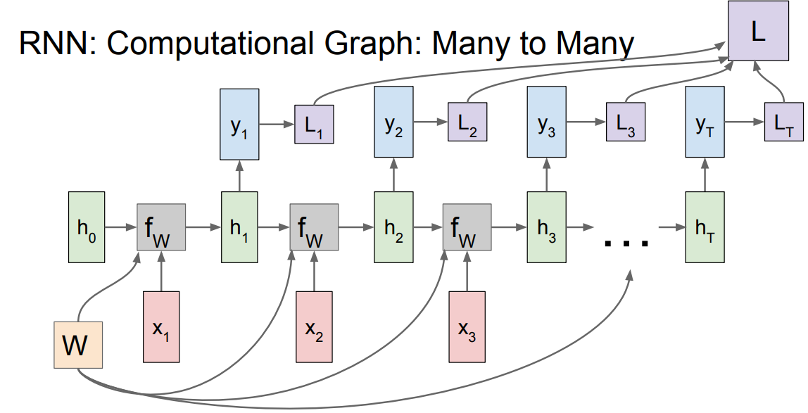
* Also the last is the sum of all losses and the weights of Y is one and is updated through summing all the gradients!
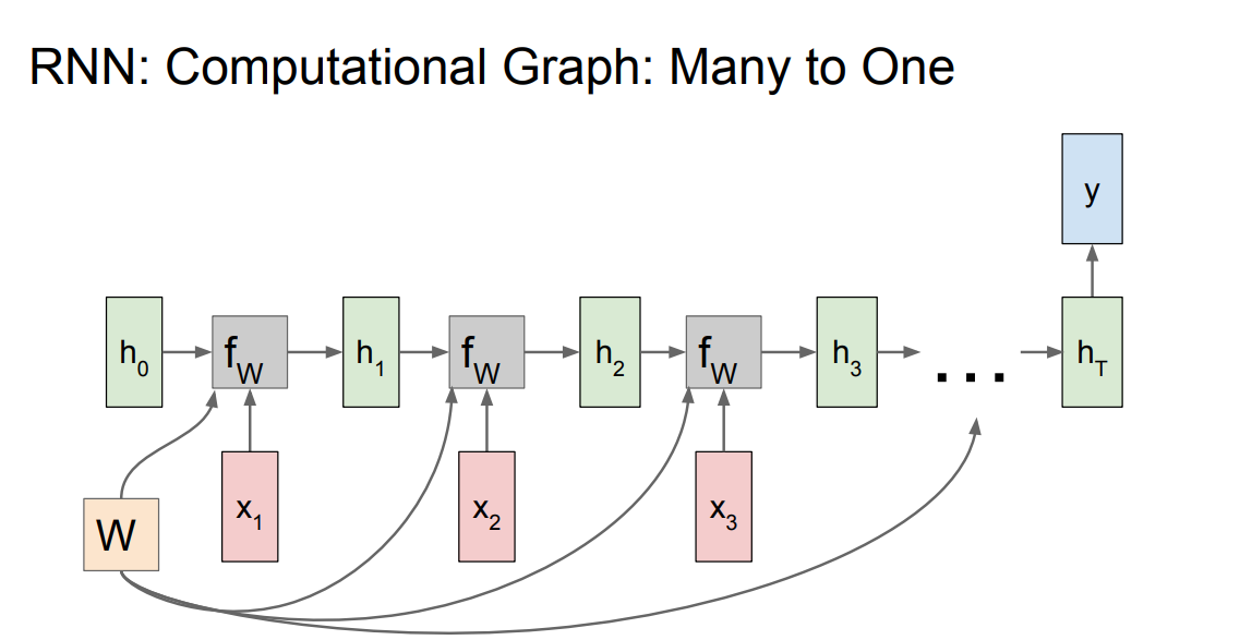
* A many to one graph:
* 
* A one to many graph:
* 
* sequence to sequence graph:
* 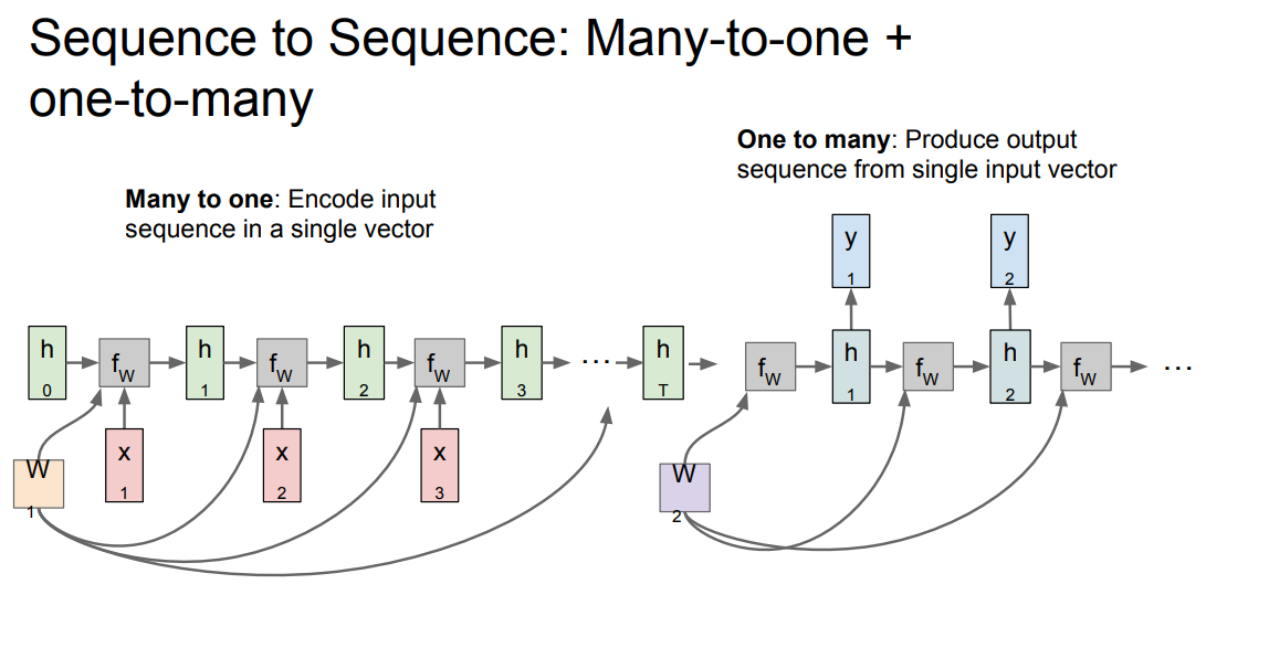
* Encoder and decoder philosophy.
* Examples:
* Suppose we are building words using characters. We want a model to predict the next character of a sequence. Lets say that the characters are only `[h, e, l, o]` and the words are \[hello]
* Training:
* 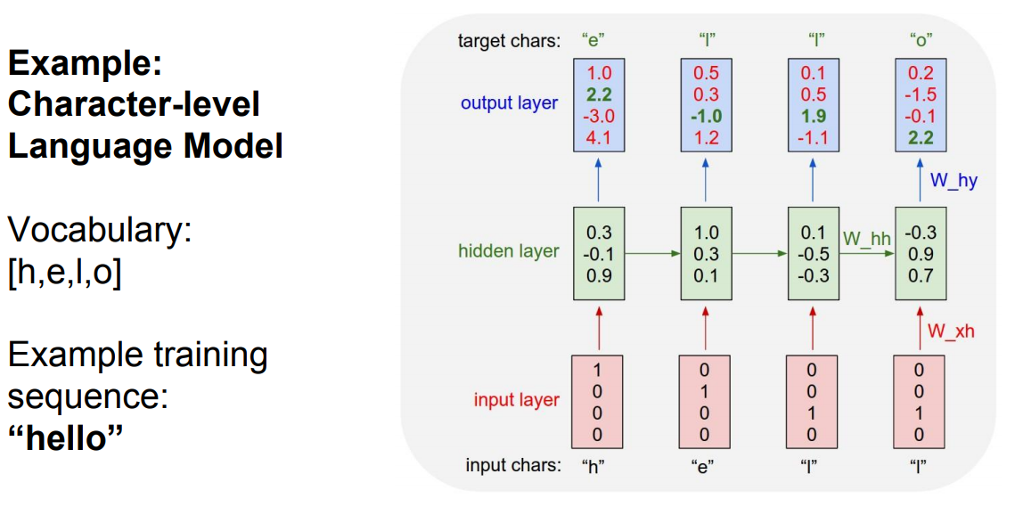
* Only the third prediction here is true. The loss needs to be optimized.
* We can train the network by feeding the whole word(s).
* Testing time:
* 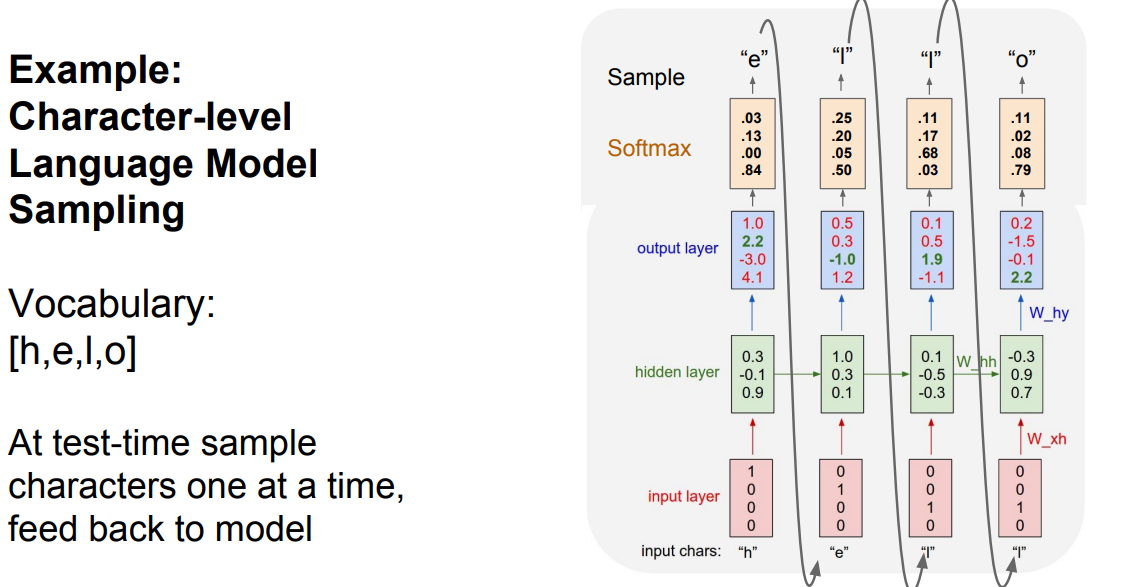
* At test time we work with a character by character. The output character will be the next input with the other saved hidden activations.
* This [link](https://gist.github.com/karpathy/d4dee566867f8291f086) contains all the code but uses Truncated Backpropagation through time as we will discuss.
* Backpropagation through time Forward through entire sequence to compute loss, then backward through entire sequence to compute gradient.
* But if we choose the whole sequence it will be so slow and take so much memory and will never converge!
* So in practice people are doing "Truncated Backpropagation through time" as we go on we Run forward and backward through chunks of the sequence instead of whole sequence
* Then Carry hidden states forward in time forever, but only backpropagate for some smaller number of steps.
* Example on image captioning:
* 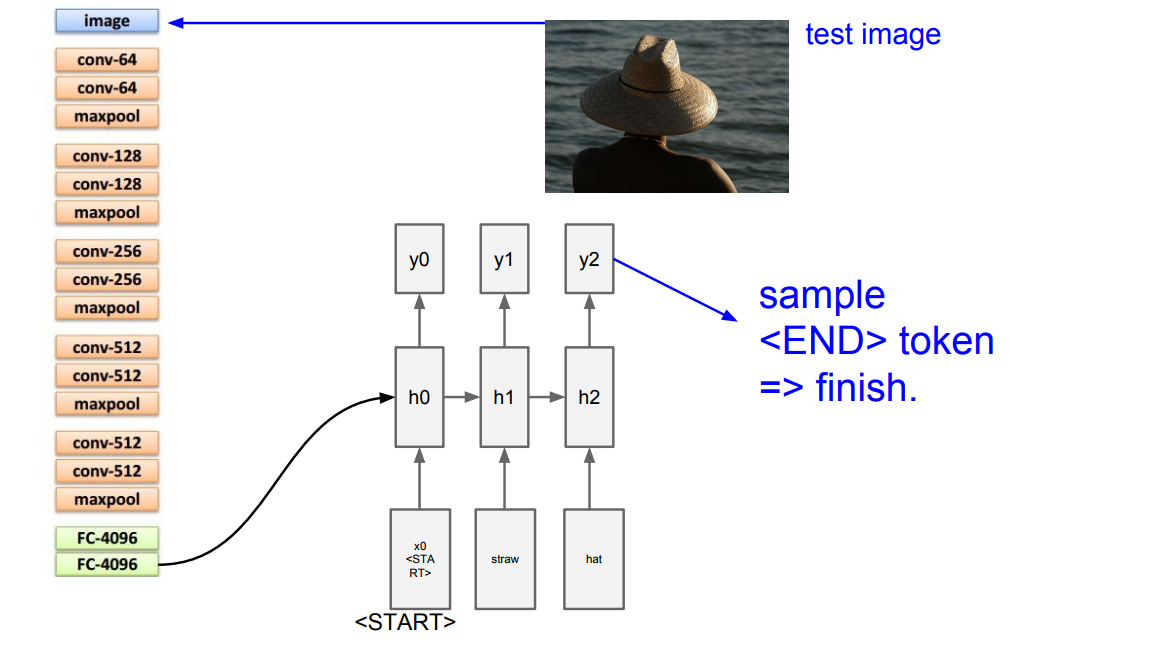
* They use token to finish running.
* The biggest dataset for image captioning is Microsoft COCO.
* Image Captioning with Attention is a project in which when the RNN is generating captions, it looks at a specific part of the image not the whole image.
* Image Captioning with Attention technique is also used in "Visual Question Answering" problem
* Multilayer RNNs is generally using some layers as the hidden layer that are feed into again. **LSTM** is a multilayer RNNs.
* Backward flow of gradients in RNN can explode or vanish. Exploding is controlled with gradient clipping. Vanishing is controlled with additive interactions (LSTM)
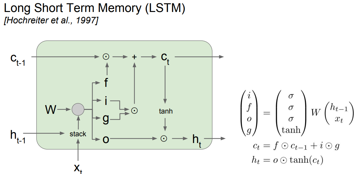
* LSTM stands for Long Short Term Memory. It was designed to help the vanishing gradient problem on RNNs.
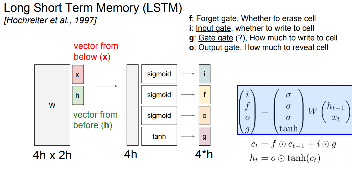
* It consists of:
* f: Forget gate, Whether to erase cell
* i: Input gate, whether to write to cell
* g: Gate gate (?), How much to write to cell
* o: Output gate, How much to reveal cell
* 
* 
* The LSTM gradients are easily computed like ResNet
* The LSTM is keeping data on the long or short memory as it trains means it can remember not just the things from last layer but layers.
* Highway networks is something between ResNet and LSTM that is still in research.
* Better/simpler architectures are a hot topic of current research
* Better understanding (both theoretical and empirical) is needed.
* RNN is used for problems that uses sequences of related inputs more. Like NLP and Speech recognition.
## 11. Detection and Segmentation
* So far we are talking about image classification problem. In this section we will talk about Segmentation, Localization, Detection.
* **Semantic Segmentation**
* We want to Label each pixel in the image with a category label.
* 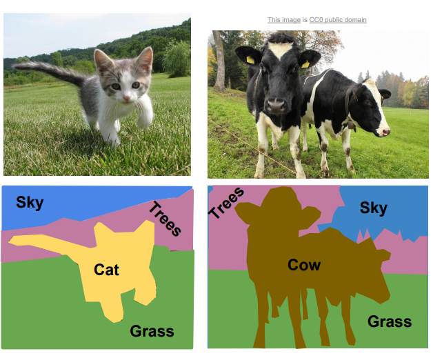
* As you see the cows in the image, Semantic Segmentation Don’t differentiate instances, only care about pixels.
* The first idea is to use a **sliding window**. We take a small window size and slide it all over the picture. For each window we want to label the center pixel.
* It will work but its not a good idea because it will be computational expensive!
* Very inefficient! Not reusing shared features between overlapping patches.
* In practice nobody uses this.
* The second idea is designing a network as a bunch of Convolutional layers to make predictions for pixels all at once!
* Input is the whole image. Output is the image with each pixel labeled.
* We need a lot of labeled data. And its very expensive data.
* It needs a deep Conv. layers.
* The loss is cross entropy between each pixel provided.
* Data augmentation are good here.
* The problem with this implementation that convolutions at original image resolution will be very expensive.
* So in practice we don't see something like this right now.
* The third idea is based on the last idea. The difference is that we are downsampling and upsampling inside the network.
* We downsample because using the whole image as it is very expensive. So we go on multiple layers downsampling and then upsampling in the end.
* Downsampling is an operation like Pooling and strided convolution.
* Upsampling is like "Nearest Neighbor" or "Bed of Nails" or "Max unpooling"
* **Nearest Neighbor** example:
```
Input: 1 2 Output: 1 1 2 2
3 4 1 1 2 2
3 3 4 4
3 3 4 4
```
```
- **Bed of Nails** example:
```
```
Input: 1 2 Output: 1 0 2 0
3 4 0 0 0 0
3 0 4 0
0 0 0 0
```
```
* **Max unpooling** is depending on the earlier steps that was made by max pooling. You fill the pixel where max pooling took place and then fill other pixels by zero.
* Max unpooling seems to be the best idea for upsampling.
* There are an idea of Learnable Upsampling called "**Transpose Convolution**"
* Rather than making a convolution we make the reverse.
* Also called:
* Upconvolution.
* Fractionally strided convolution
* Backward strided convolution
* Learn the artimitic of the upsampling please refer to chapter 4 in this [paper](https://arxiv.org/abs/1603.07285).
```
* **Classification + Localization**:
* In this problem we want to classify the main object in the image and its location as a rectangle.
* We assume there are one object.
* We will create a multi task NN. The architecture are as following:
* Convolution network layers connected to:
* FC layers that classify the object. `# The plain classification problem we know`
* FC layers that connects to a four numbers `(x,y,w,h)`
* We treat Localization as a regression problem.
* This problem will have two losses:
* Softmax loss for classification
* Regression (Linear loss) for the localization (L2 loss)
* Loss = SoftmaxLoss + L2 loss
* Often the first Conv layers are pretrained NNs like AlexNet!
* This technique can be used in so many other problems like: Human Pose Estimation.
* **Object Detection**
* A core idea of computer vision. We will talk by details in this problem.
* The difference between "Classification + Localization" and this problem is that here we want to detect one or mode different objects and its locations!
* First idea is to use a sliding window
* Worked well and long time.
* The steps are:
* Apply a CNN to many different crops of the image, CNN classifies each crop as object or background.
* The problem is we need to apply CNN to huge number of locations and scales, very computationally expensive!
* The brute force sliding window will make us take thousands of thousands of time.
* Region Proposals will help us deciding which region we should run our NN at:
* Find **blobby** image regions that are likely to contain objects.
* Relatively fast to run; e.g. Selective Search gives 1000 region proposals in a few seconds on CPU
* So now we can apply one of the Region proposals networks and then apply the first idea.
* There is another idea which is called R-CNN
* 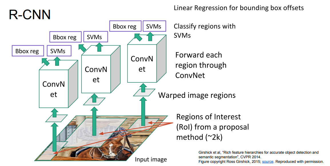
* The idea is bad because its taking parts of the image -With Region Proposalsif different sizes and feed it to CNN after scaling them all to one size. Scaling is bad
* Also its very slow.
* Fast R-CNN is another idea that developed on R-CNN
* 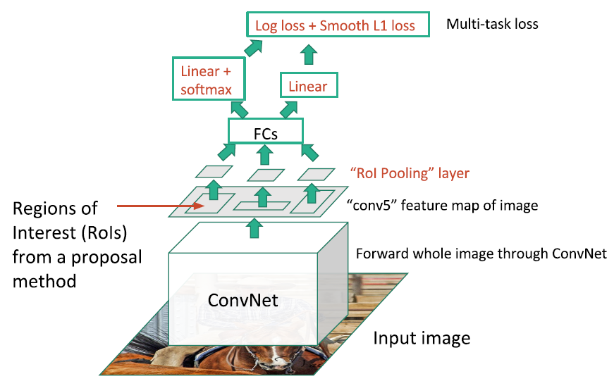
* It uses one CNN to do everything.
* Faster R-CNN does its own region proposals by Inserting Region Proposal Network (RPN) to predict proposals from features.
* The fastest of the R-CNNs.
* Another idea is Detection without Proposals: YOLO / SSD
* YOLO stands for you only look once.
* YOLO/SDD is two separate algorithms.
* Faster but not as accurate.
* Takeaways
* Faster R-CNN is slower but more accurate.
* SSD/YOLO is much faster but not as accurate.
* **Denese Captioning**
* Denese Captioning is "Object Detection + Captioning"
* Paper that covers this idea can be found [here](https://arxiv.org/abs/1511.07571).
* **Instance Segmentation**
* This is like the full problem.
* 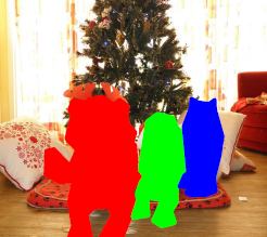
* Rather than we want to predict the bounding box, we want to know which pixel label but also distinguish them.
* There are a lot of ideas.
* There are a new idea "Mask R-CNN"
* Like R-CNN but inside it we apply the Semantic Segmentation
* There are a lot of good results out of this paper.
* It sums all the things that we have discussed in this lecture.
* Performance of this seems good.
## 12. Visualizing and Understanding
* We want to know what’s going on inside ConvNets?
* People want to trust the black box (CNN) and know how it exactly works and give and good decisions.
* A first approach is to visualize filters of the first layer.
* Maybe the shape of the first layer filter is 5 x 5 x 3, and the number of filters are 16. Then we will have 16 different "colored" filter images.
* It turns out that these filters learns primitive shapes and oriented edges like the human brain does.
* These filters really looks the same on each Conv net you will train, Ex if you tried to get it out of AlexNet, VGG, GoogleNet, or ResNet.
* This will tell you what is the first convolution layer is looking for in the image.
* We can visualize filters from the next layers but they won't tell us anything.
* Maybe the shape of the first layer filter is 5 x 5 x 20, and the number of filters are 16. Then we will have 16\*20 different "gray" filter images.
* In AlexNet, there was some FC layers in the end. If we took the 4096-dimensional feature vector for an image, and collecting these feature vectors.
* If we made a nearest neighbors between these feature vectors and get the real images of these features we will get something very good compared with running the KNN on the images directly!
* 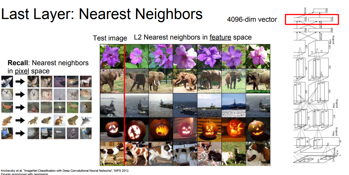
* This similarity tells us that these CNNs are really getting the semantic meaning of these images instead of on the pixels level!
* We can make a dimensionality reduction on the 4096 dimensional feature and compress it to 2 dimensions.
* This can be made by PCA, or t-SNE.
* t-SNE are used more with deep learning to visualize the data. Example can be found [here](http://cs.stanford.edu/people/karpathy/cnnembed/).
* We can Visualize the activation maps.
* For example if CONV5 feature map is 128 x 13 x 13, We can visualize it as 128 13 x 13 gray-scale images.
* 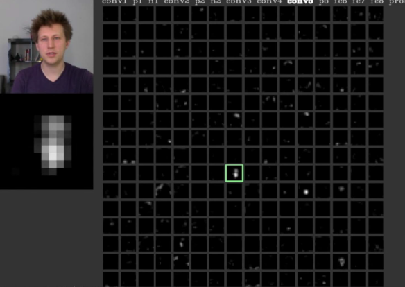
* One of these features are activated corresponding to the input, so now we know that this particular map are looking for something.
* Its done by Yosinski et. More info are [here](http://yosinski.com/deepvis#toolbox).
* There are something called **Maximally Activating Patches** that can help us visualize the intermediate features in Convnets
* The steps of doing this is as following:
* We choose a layer then a neuron
* Ex. We choose Conv5 in AlexNet which is 128 x 13 x 13 then pick channel (Neuron) 17/128
* Run many images through the network, record values of chosen channel.
* Visualize image patches that correspond to maximal activations.
* We will find that each neuron is looking into a specific part of the image.
* Extracted images are extracted using receptive field.
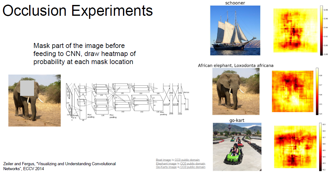
* Another idea is **Occlusion Experiments**
* We mask part of the image before feeding to CNN, draw heat-map of probability (Output is true) at each mask location
* It will give you the most important parts of the image in which the Conv. Network has learned from.
* 
* **Saliency Maps** tells which pixels matter for classification
* Like Occlusion Experiments but with a completely different approach
* We Compute gradient of (unnormalized) class score with respect to image pixels, take absolute value and max over RGB channels. It will get us a gray image that represents the most important areas in the image.
* This can be used for Semantic Segmentation sometimes.
* (guided) backprop Makes something like **Maximally Activating Patches** but unlike it gets the pixels in which we are caring of.
* In this technique choose a channel like Maximally Activating Patches and then compute gradient of neuron value with respect to image pixels
* Images come out nicer if you only backprop positive gradients through each RELU (guided backprop)
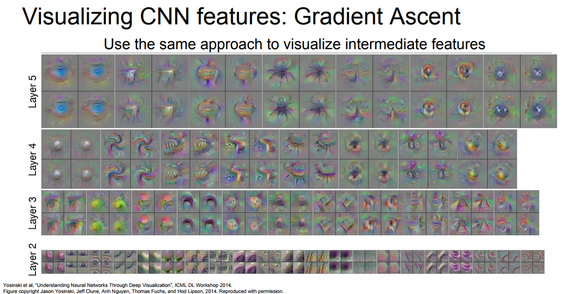
* **Gradient Ascent**
* Generate a synthetic image that maximally activates a neuron.
* Reverse of gradient decent. Instead of taking the minimum it takes the maximum.
* We want to maximize the neuron with the input image. So here instead we are trying to learn the image that maximize the activation:
\*
* ```python
# R(I) is Natural image regularizer, f(I) is the neuron value.
I *= argmax(f(I)) + R(I)
```
*
* Steps of gradient ascent
* Initialize image to zeros.
* Forward image to compute current scores.
* Backprop to get gradient of neuron value with respect to image pixels.
* Make a small update to the image
* `R(I)` may equal to L2 of generated image.
* To get a better results we use a better regularizer:
* penalize L2 norm of image; also during optimization periodically:
* Gaussian blur image
* Clip pixels with small values to 0
* Clip pixels with small gradients to 0
* A better regularizer makes out images cleaner!
*
```
```
* The results in the latter layers seems to mean something more than the other layers.
* We can fool CNN by using this procedure:
* Start from an arbitrary image. `# Random picture based on nothing.`
* Pick an arbitrary class. `# Random class`
* Modify the image to maximize the class.
* Repeat until network is fooled.
* Results on fooling the network is pretty surprising!
* 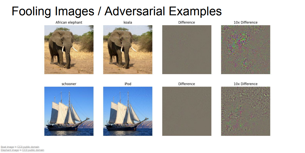
* For human eyes they are the same, but it fooled the network by adding just some noise!
* **DeepDream**: Amplify existing features
* Google released deep dream on their website.
* What its actually doing is the same procedure as fooling the NN that we discussed, but rather than synthesizing an image to maximize a specific neuron, instead try to amplify the neuron activations at some layer in the network.
* Steps:
* Forward: compute activations at chosen layer. `# form an input image (Any image)`
* Set gradient of chosen layer equal to its activation.
* Equivalent to `I* = arg max[I] sum(f(I)^2)`
* Backward: Compute gradient on image.
* Update image.
* The code of deep dream is online you can download and check it yourself.
* **Feature Inversion**
* Gives us to know what types of elements parts of the image are captured at different layers in the network.
* Given a CNN feature vector for an image, find a new image that:
* Matches the given feature vector.
* *looks natural* (image prior regularization)
* **Texture Synthesis**
* Old problem in computer graphics.
* Given a sample patch of some texture, can we generate a bigger image of the same texture?
* There is an algorithm which doesn't depend on NN:
* Wei and Levoy, Fast Texture Synthesis using Tree-structured Vector Quantization, SIGGRAPH 2000
* Its a really simple algorithm
* The idea here is that this is an old problem and there are a lot of algorithms that has already solved it but simple algorithms doesn't work well on complex textures!
* An idea of using NN has been proposed on 2015 based on gradient ascent and called it "Neural Texture Synthesis"
* It depends on something called Gram matrix.
* Neural Style Transfer = Feature + Gram Reconstruction
* Gatys, Ecker, and Bethge, Image style transfer using Convolutional neural networks, CVPR 2016
* Implementation by pytorch [here](https://github.com/jcjohnson/neural-style).
* Style transfer requires many forward / backward passes through VGG; very slow!
* Train another neural network to perform style transfer for us!
* Fast Style Transfer is the solution.
* Johnson, Alahi, and Fei-Fei, Perceptual Losses for Real-Time Style Transfer and Super-Resolution, ECCV 2016
*
* There are a lot of work on these style transfer and it continues till now!
* Summary:
* Activations: Nearest neighbors, Dimensionality reduction, maximal patches, occlusion
* Gradients: Saliency maps, class visualization, fooling images, feature inversion
* Fun: DeepDream, Style Transfer
## 13. Generative models
* Generative models are type of Unsupervised learning.
* Supervised vs Unsupervised Learning:
* | | Supervised Learning | Unsupervised Learning |
| -------------- | ------------------------------------------------------------------------------------- | -------------------------------------------------------------------------- |
| Data structure | Data: (x, y), and x is data, y is label | Data: x, Just data, no labels! |
| Data price | Training data is expensive in a lot of cases. | Training data are cheap! |
| Goal | Learn a function to map x -> y | Learn some underlying hidden structure of the data |
| Examples | Classification, regression, object detection, semantic segmentation, image captioning | Clustering, dimensionality reduction, feature learning, density estimation |
* Autoencoders are a Feature learning technique.
* 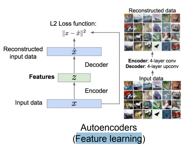
* It contains an encoder and a decoder. The encoder downsamples the image while the decoder upsamples the features.
* The loss are L2 loss.
* Density estimation is where we want to learn/estimate the underlaying distribution for the data!
* There are a lot of research open problems in unsupervised learning compared with supervised learning!
* **Generative Models**
* Given training data, generate new samples from same distribution.
* Addresses density estimation, a core problem in unsupervised learning.
* We have different ways to do this:
* Explicit density estimation: explicitly define and solve for the learning model.
* Learn model that can sample from the learning model without explicitly defining it.
* Why Generative Models?
* Realistic samples for artwork, super-resolution, colorization, etc
* Generative models of time-series data can be used for simulation and planning (reinforcement learning applications!)
* Training generative models can also enable inference of latent representations that can be useful as general features
* Taxonomy of Generative Models:
* 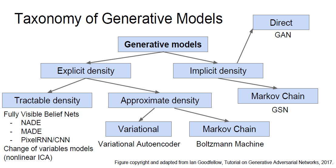
* In this lecture we will discuss: PixelRNN/CNN, Variational Autoencoder, and GANs as they are the popular models in research now.
* **PixelRNN** and **PixelCNN**
* In a full visible belief network we use the chain rule to decompose likelihood of an image x into product of 1-d distributions
* `p(x) = sum(p(x[i]| x[1]x[2]....x[i-1]))`
* Where p(x) is the Likelihood of image x and x\[i] is Probability of i’th pixel value given all previous pixels.
* To solve the problem we need to maximize the likelihood of training data but the distribution is so complex over pixel values.
* Also we will need to define ordering of previous pixels.
* PixelRNN
* Founded by \[van der Oord et al. 2016]
* Dependency on previous pixels modeled using an RNN (LSTM)
* Generate image pixels starting from corner
* Drawback: sequential generation is slow! because you have to generate pixel by pixel!
* PixelCNN
* Also Founded by \[van der Oord et al. 2016]
* Still generate image pixels starting from corner.
* Dependency on previous pixels now modeled using a CNN over context region
* Training is faster than PixelRNN (can parallelize convolutions since context region values known from training images)
* Generation must still proceed sequentially still slow.
* There are some tricks to improve PixelRNN & PixelCNN.
* PixelRNN and PixelCNN can generate good samples and are still active area of research.
* **Autoencoders**
* Unsupervised approach for learning a lower-dimensional feature representation from unlabeled training data.
* Consists of Encoder and decoder.
* The encoder:
* Converts the input x to the features z. z should be smaller than x to get only the important values out of the input. We can call this dimensionality reduction.
* The encoder can be made with:
* Linear or non linear layers (earlier days days)
* Deep fully connected NN (Then)
* RELU CNN (Currently we use this on images)
* The decoder:
* We want the encoder to map the features we have produced to output something similar to x or the same x.
* The decoder can be made with the same techniques we made the encoder and currently it uses a RELU CNN.
* The encoder is a conv layer while the decoder is deconv layer! Means Decreasing and then increasing.
* The loss function is L2 loss function:
* `L[i] = |y[i] - y'[i]|^2`
* After training we though away the decoder.`# Now we have the features we need`
* We can use this encoder we have to make a supervised model.
* The value of this it can learn a good feature representation to the input you have.
* A lot of times we will have a small amount of data to solve problem. One way to tackle this is to use an Autoencoder that learns how to get features from images and train your small dataset on top of that model.
* The question is can we generate data (Images) from this Autoencoder?
* **Variational Autoencoders (VAE)**
* Probabilistic spin on Autoencoders - will let us sample from the model to generate data!
* We have z as the features vector that has been formed using the encoder.
* We then choose prior p(z) to be simple, e.g. Gaussian.
* Reasonable for hidden attributes: e.g. pose, how much smile.
* Conditional p(x|z) is complex (generates image) => represent with neural network
* But we cant compute integral for P(z)p(x|z)dz as the following equation:
* 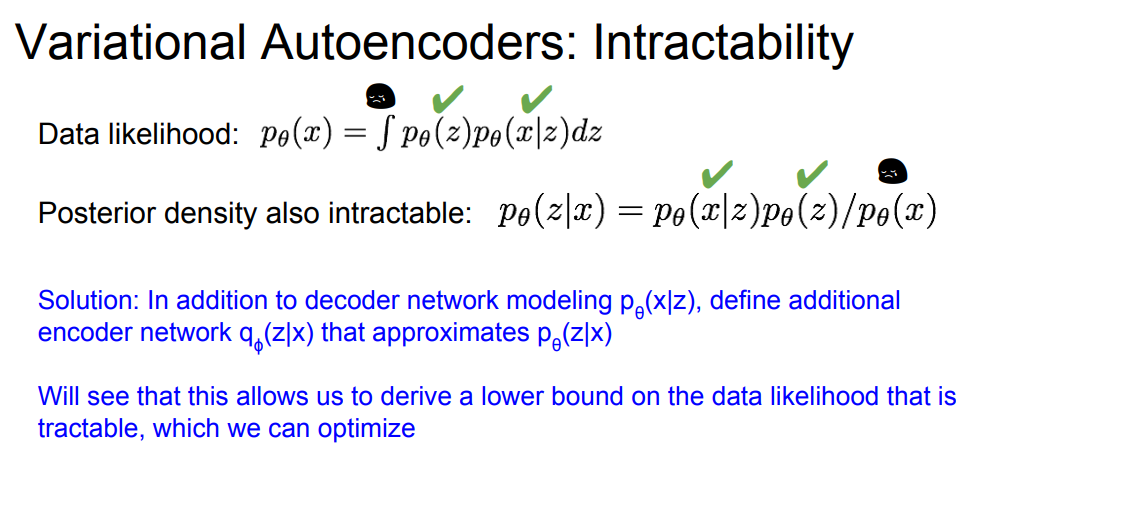
* After resolving all the equations that solves the last equation we should get this:
* 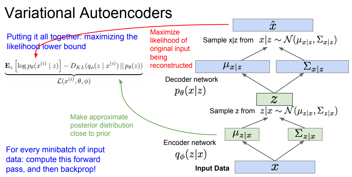
* Variational Autoencoder are an approach to generative models but Samples blurrier and lower quality compared to state-of-the-art (GANs)
* Active areas of research:
* More flexible approximations, e.g. richer approximate posterior instead of diagonal Gaussian
* Incorporating structure in latent variables
* **Generative Adversarial Networks (GANs)**
* GANs don’t work with any explicit density function!
* Instead, take game-theoretic approach: learn to generate from training distribution through 2-player game.
* Yann LeCun, who oversees AI research at Facebook, has called GANs:
* > The coolest idea in deep learning in the last 20 years
* Problem: Want to sample from complex, high-dimensional training distribution. No direct way to do this as we have discussed!
* Solution: Sample from a simple distribution, e.g. random noise. Learn transformation to training distribution.
* So we create a noise image which are drawn from simple distribution feed it to NN we will call it a generator network that should learn to transform this into the distribution we want.
* Training GANs: Two-player game:
* **Generator network**: try to fool the discriminator by generating real-looking images.
* **Discriminator network**: try to distinguish between real and fake images.
* If we are able to train the Discriminator well then we can train the generator to generate the right images.
* The loss function of GANs as minimax game are here:
* 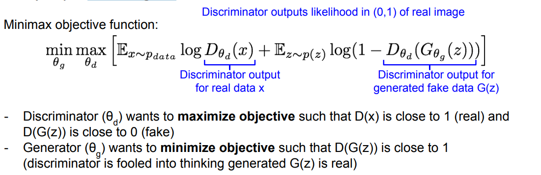
* The label of the generator network will be 0 and the real images are 1.
* To train the network we will do:
* Gradient ascent on discriminator.
* Gradient ascent on generator but with different loss.
* You can read the full algorithm with the equations here:
* 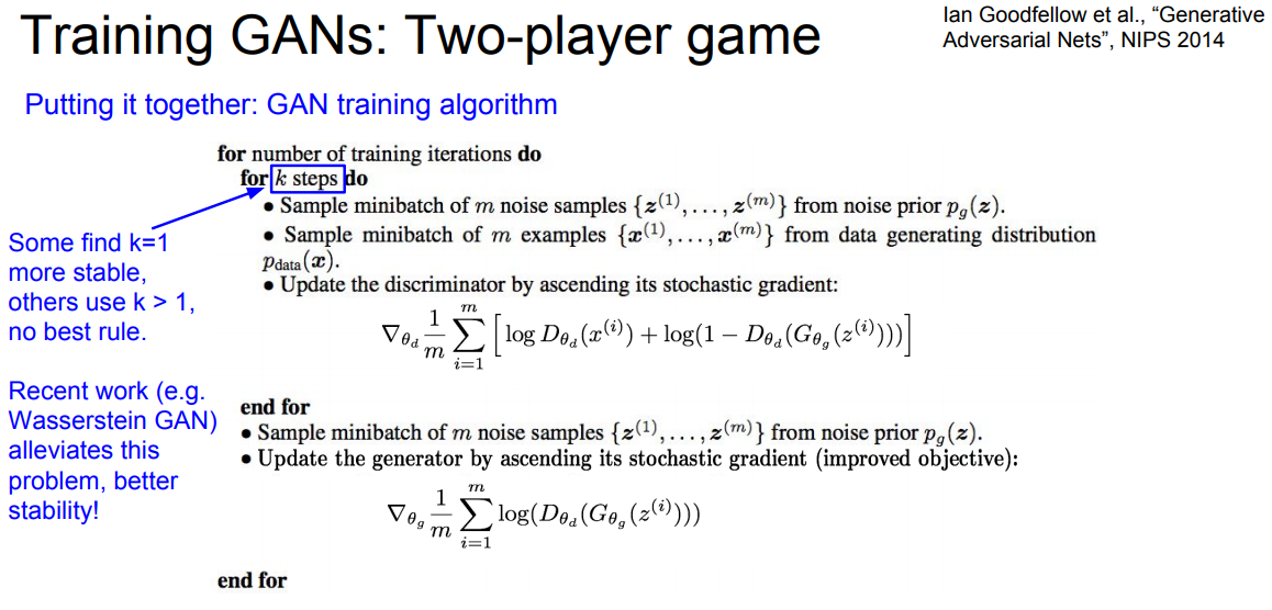
* Aside: Jointly training two networks is challenging, can be unstable. Choosing objectives with better loss landscapes helps training is an active area of research.
* Convolutional Architectures:
* Generator is an upsampling network with fractionally-strided convolutions Discriminator is a Convolutional network.
* Guidelines for stable deep Conv GANs:
* Replace any pooling layers with strided convs (discriminator) and fractional-strided convs with (Generator).
* Use batch norm for both networks.
* Remove fully connected hidden layers for deeper architectures.
* Use RELU activation in generator for all layers except the output which uses Tanh
* Use leaky RELU in discriminator for all the layers.
* 2017 is the year of the GANs! it has exploded and there are some really good results.
* Active areas of research also is GANs for all kinds of applications.
* The GAN zoo can be found here:
* Tips and tricks for using GANs:
* NIPS 2016 Tutorial GANs:
## 14. Deep reinforcement learning
* This section contains a lot of math.
* Reinforcement learning problems are involving an agent interacting with an environment, which provides numeric reward signals.
* Steps are:
* Environment --> State `s[t]` --> Agent --> Action `a[t]` --> Environment --> `Reward r[t]` + Next state `s[t+1]` --> Agent --> and so on..
* Our goal is learn how to take actions in order to maximize reward.
* An example is Robot Locomotion:
* Objective: Make the robot move forward
* State: Angle and position of the joints
* Action: Torques applied on joints
* 1 at each time step upright + forward movement
* Another example is Atari Games:
* Deep learning has a good state of art in this problem.
* Objective: Complete the game with the highest score.
* State: Raw pixel inputs of the game state.
* Action: Game controls e.g. Left, Right, Up, Down
* Reward: Score increase/decrease at each time step
* Go game is another example which AlphaGo team won in the last year (2016) was a big achievement for AI and deep learning because the problem was so hard.
* We can mathematically formulate the RL (reinforcement learning) by using **Markov Decision Process**
* **Markov Decision Process**
* Defined by (`S`, `A`, `R`, `P`, `Y`) where:
* `S`: set of possible states.
* `A`: set of possible actions
* `R`: distribution of reward given (state, action) pair
* `P`: transition probability i.e. distribution over next state given (state, action) pair
* `Y`: discount factor `# How much we value rewards coming up soon verses later on.`
* Algorithm:
* At time step `t=0`, environment samples initial state `s[0]`
* Then, for t=0 until done:
* Agent selects action `a[t]`
* Environment samples reward from `R` with (`s[t]`, `a[t]`)
* Environment samples next state from `P` with (`s[t]`, `a[t]`)
* Agent receives reward `r[t]` and next state `s[t+1]`
* A policy `pi` is a function from S to A that specifies what action to take in each state.
* Objective: find policy `pi*` that maximizes cumulative discounted reward: `Sum(Y^t * r[t], t>0)`
* For example:
* 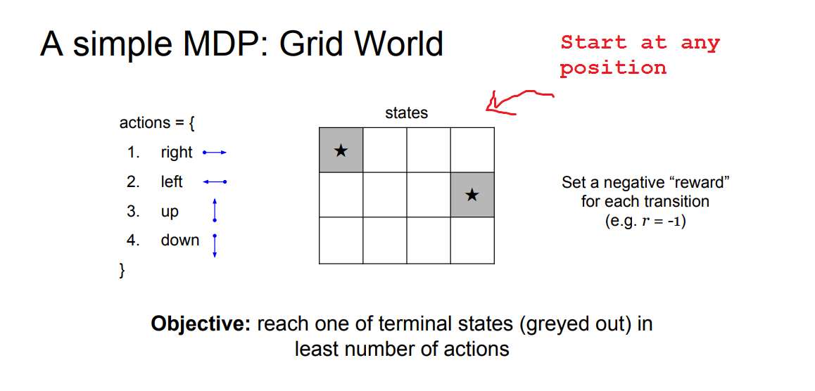
* Solution would be:
* 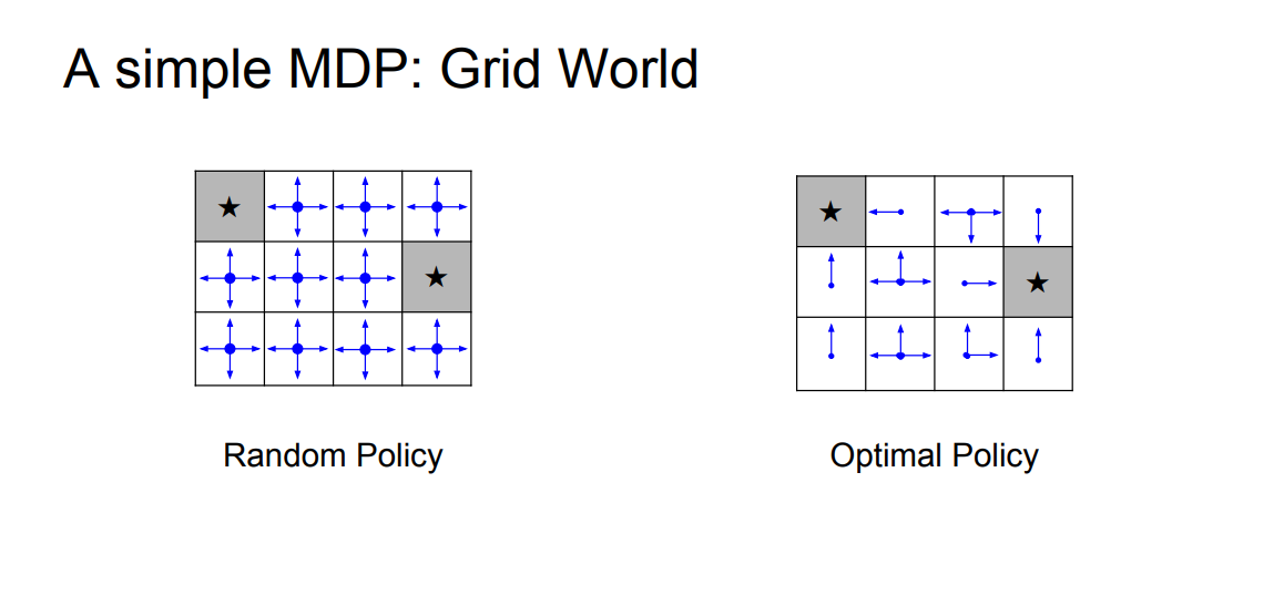
* The value function at state `s`, is the expected cumulative reward from following the policy from state `s`:
* `V[pi](s) = Sum(Y^t * r[t], t>0) given s0 = s, pi`
* The Q-value function at state s and action `a`, is the expected cumulative reward from taking action `a` in state `s` and then following the policy:
* `Q[pi](s,a) = Sum(Y^t * r[t], t>0) given s0 = s,a0 = a, pi`
* The optimal Q-value function `Q*` is the maximum expected cumulative reward achievable from a given (state, action) pair:
* `Q*[s,a] = Max(for all of pi on (Sum(Y^t * r[t], t>0) given s0 = s,a0 = a, pi))`
* Bellman equation
* Important thing is RL.
* Given any state action pair (s,a) the value of this pair is going to be the reward that you are going to get r plus the value of the state that you end in.
* `Q*[s,a] = r + Y * max Q*(s',a') given s,a # Hint there is no policy in the equation`
* The optimal policy `pi*` corresponds to taking the best action in any state as specified by `Q*`
* We can get the optimal policy using the value iteration algorithm that uses the Bellman equation as an iterative update
* 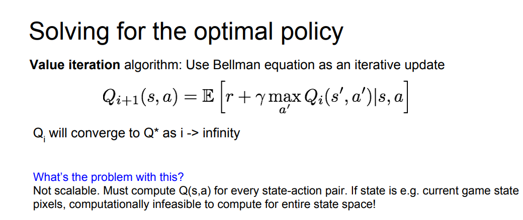
* Due to the huge space dimensions in real world applications we will use a function approximator to estimate `Q(s,a)`. E.g. a neural network! this is called **Q-learning**
* Any time we have a complex function that we cannot represent we use Neural networks!
* **Q-learning**
* The first deep learning algorithm that solves the RL.
* Use a function approximator to estimate the action-value function
* If the function approximator is a deep neural network => deep q-learning
* The loss function:
* 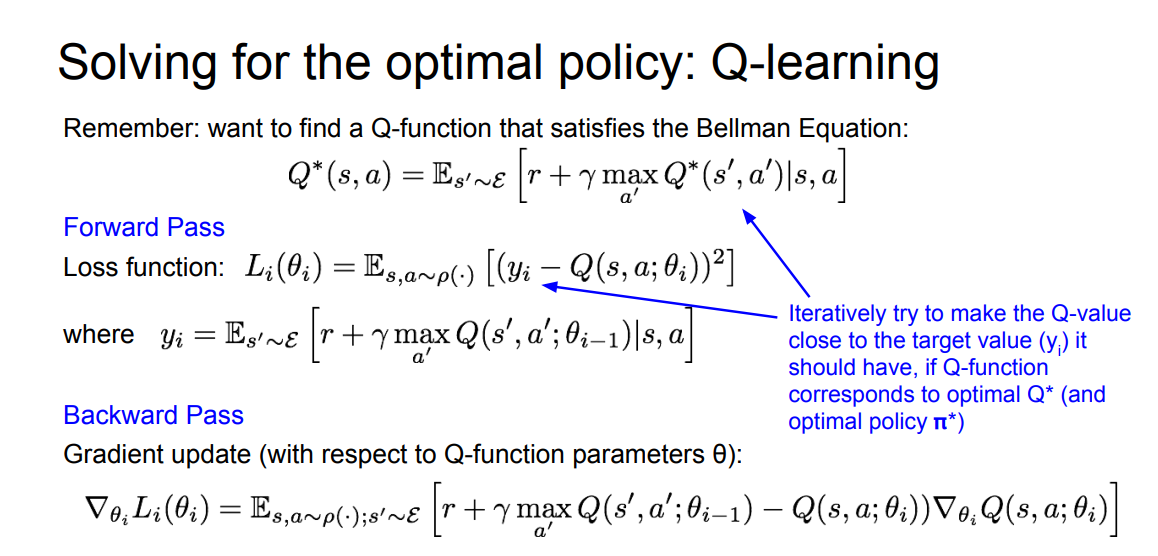
* Now lets consider the "Playing Atari Games" problem:
* Our total reward are usually the reward we are seeing in the top of the screen.
* Q-network Architecture:
* 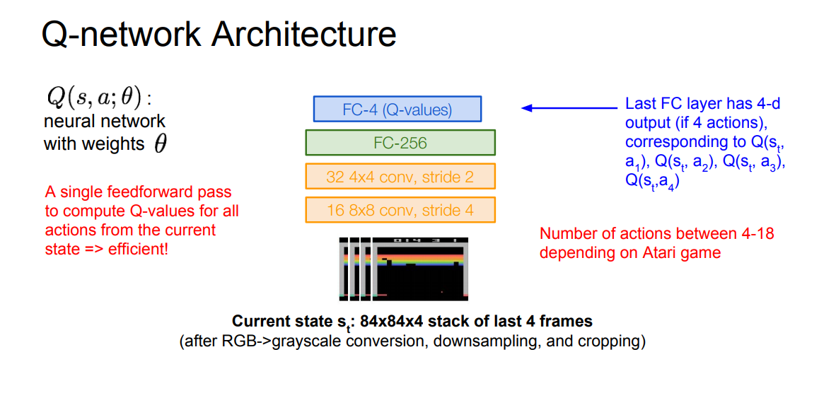
* Learning from batches of consecutive samples is a problem. If we recorded a training data and set the NN to work with it, if the data aren't enough we will go to a high bias error. so we should use "experience replay" instead of consecutive samples where the NN will try the game again and again until it masters it.
* Continually update a replay memory table of transitions (`s[t]` , `a[t]` , `r[t]` , `s[t+1]`) as game (experience) episodes are played.
* Train Q-network on random minibatches of transitions from the replay memory, instead of consecutive samples.
* The full algorithm:
* 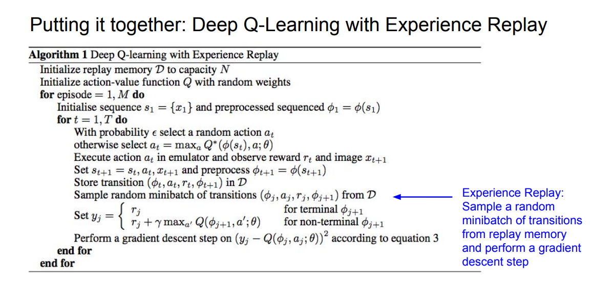
* A video that demonstrate the algorithm on Atari game can be found here: ""
* **Policy Gradients**
* The second deep learning algorithm that solves the RL.
* The problem with Q-function is that the Q-function can be very complicated.
* Example: a robot grasping an object has a very high-dimensional state.
* But the policy can be much simpler: just close your hand.
* Can we learn a policy directly, e.g. finding the best policy from a collection of policies?
* Policy Gradients equations:
* 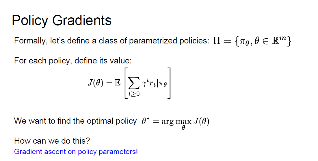
* Converges to a local minima of `J(ceta)`, often good enough!
* REINFORCE algorithm is the algorithm that will get/predict us the best policy
* Equation and intuition of the Reinforce algorithm:
* 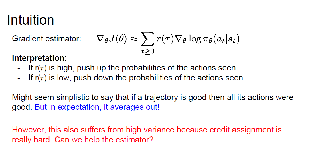
* the problem was high variance with this equation can we solve this?
* variance reduction is an active research area!
* Recurrent Attention Model (RAM) is an algorithm that are based on REINFORCE algorithm and is used for image classification problems:
* Take a sequence of “glimpses” selectively focusing on regions of the image, to predict class
* Inspiration from human perception and eye movements.
* Saves computational resources => scalability
* If an image with high resolution you can save a lot of computations
* Able to ignore clutter / irrelevant parts of image
* RAM is used now in a lot of tasks: including fine-grained image recognition, image captioning, and visual question-answering
* AlphaGo are using a mix of supervised learning and reinforcement learning, It also using policy gradients.
* A good course from Standford on deep reinforcement learning
*
*
* A good course on deep reinforcement learning (2017)
*
*
* A good article
*
## 15. Efficient Methods and Hardware for Deep Learning
* The original lecture was given by Song Han a PhD Candidate at standford.
* Deep Conv nets, Recurrent nets, and deep reinforcement learning are shaping a lot of applications and changing a lot of our lives.
* Like self driving cars, machine translations, alphaGo and so on.
* But the trend now says that if we want a high accuracy we need a larger (Deeper) models.
* The model size in ImageNet competation from 2012 to 2015 has increased 16x to achieve a high accurecy.
* Deep speech 2 has 10x training operations than deep speech 1 and thats in only one year! `# At Baidu`
* There are three challenges we got from this
* **Model Size**
* Its hard to deploy larger models on our PCs, mobiles, or cars.
* **Speed**
* ResNet152 took 1.5 weeks to train and give the 6.16% accurecy!
* Long training time limits ML researcher’s productivity
* **Energy Efficiency**
* AlphaGo: 1920 CPUs and 280 GPUs. $3000 electric bill per game
* If we use this on our mobile it will drain the battery.
* Google mentioned in thier blog if all the users used google speech for 3 minutes, they have to double thier data-center!
* Where is the Energy Consumed?
* larger model => more memory reference => more energy
* We can improve the Efficiency of Deep Learning by Algorithm-Hardware Co-Design.
* From both the hardware and the algorithm perspectives.
* Hardware 101: the Family
* **General Purpose** `# Used for any hardware`
* CPU `# Latency oriented, Single strong threaded like a single elepahnt`
* GPU `# Throughput oriented, So many small threads like a lot of ants`
* GPGPU
* **Specialized HW** `#Tuned for a domain of applications`
* FPGA# Programmable logic, Its cheaper but less effiecnet\`
* ASIC`# Fixed logic, Designed for a certian applications (Can be designed for deep learning applications)`
* Hardware 101: Number Representation
* Numbers in computer are represented with a discrete memory.
* Its very good and energy efficent for hardware to go from 32 bit to 16 bit in float point operations.
* Part 1: **Algorithms for Efficient Inference**
* **Pruning neural networks**
* Idea is can we remove some of the weights/neurons and the NN still behave the same?
* In 2015 Han made AlexNet parameters from 60 million to 6 Million! by using the idea of Pruning.
* Pruning can be applied to CNN and RNN, iteratively it will reach the same accurecy as the original.
* Pruning actually happends to humans:
* Newborn(50 Trillion Synapses) ==> 1 year old(1000 Trillion Synapses) ==> Adolescent(500 Trillion Synapses)
* Algorithm:
1. Get Trained network.
2. Evaluate importance of neurons.
3. Remove the least important neuron.
4. Fine tune the network.
5. If we need to continue Pruning we go to step 2 again else we stop.
* **Weight Sharing**
* The idea is that we want to make the numbers is our models less.
* Trained Quantization:
* Example: all weight values that are 2.09, 2.12, 1.92, 1.87 will be replaced by 2
* To do that we can make k means clustering on a filter for example and reduce the numbers in it. By using this we can also reduce the number of operations that are used from calculating the gradients.
* After Trained Quantization the Weights are Discrete.
* Trained Quantization can reduce the number of bits we need for a number in each layer significantly.
* Pruning + Trained Quantization can Work Together to reduce the size of the model.
* Huffman Coding
* We can use Huffman Coding to reduce/compress the number of bits of the weight.
* In-frequent weights: use more bits to represent.
* Frequent weights: use less bits to represent.
* Using Pruning + Trained Quantization + Huffman Coding is called deep compression.
* 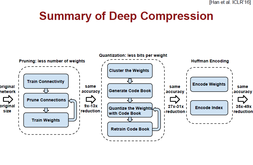
* 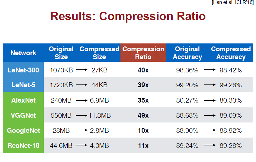
* **SqueezeNet**
* All the models we have talked about till now was using a pretrained models. Can we make a new arcitecutre that saves memory and computations?
* SqueezeNet gets the alexnet accurecy with 50x fewer parameters and 0.5 model size.
* SqueezeNet can even be further compressed by applying deep compression on them.
* Models are now more energy efficient and has speed up a lot.
* Deep compression was applied in Industry through facebook and Baidu.
* **Quantization**
* Algorithm (Quantizing the Weight and Activation):
* Train with float.
* Quantizing the weight and activation:
* Gather the statistics for weight and activation.
* Choose proper radix point position.
* Fine-tune in float format.
* Convert to fixed-point format.
* **Low Rank Approximation**
* Is another size reduction algorithm that are used for CNN.
* Idea is decompose the conv layer and then try both of the composed layers.
* **Binary / Ternary Net**
* Can we only use three numbers to represent weights in NN?
* The size will be much less with only -1, 0, 1.
* This is a new idea that was published in 2017 "Zhu, Han, Mao, Dally. Trained Ternary Quantization, ICLR’17"
* Works after training.
* They have tried it on AlexNet and it has reached almost the same error as AlexNet.
* Number of operation will increase per register:
* **Winograd Transformation**
* Based on 3x3 WINOGRAD Convolutions which makes less operations than the ordiany convolution
* cuDNN 5 uses the WINOGRAD Convolutions which has improved the speed.
* Part 2: **Hardware for Efficient Inference**
* There are a lot of ASICs that we developed for deep learning. All in which has the same goal of minimize memory access.
* Eyeriss MIT
* DaDiannao
* TPU Google (Tensor processing unit)
* It can be put to replace the disk in the server.
* Up to 4 cards per server.
* Power consumed by this hardware is a lot less than a GPU and the size of the chip is less.
* EIE Standford
* By Han at 2016 \[et al. ISCA’16]
* We don't save zero weights and make quantization for the numbers from the hardware.
* He says that EIE has a better Throughput and energy efficient.
* Part 3: **Algorithms for Efficient Training**
* **Parallelization**
* **Data Parallel**–Run multiple inputs in parallel
* Ex. Run two images in the same time!
* Run multiple training examples in parallel.
* Limited by batch size.
* Gradients have to be applied by a master node.
* **Model Parallel**
* Split up the Model–i.e. the network
* Split model over multiple processors By layer.
* Hyper-Parameter Parallel
* Try many alternative networks in parallel.
* Easy to get 16-64 GPUs training one model in parallel.
* **Mixed Precision** with FP16 and FP32
* We have discussed that if we use 16 bit real numbers all over the model the energy cost will be less by x4.
* Can we use a model entirely with 16 bit number? We can partially do this with mixed FP16 and FP32. We use 16 bit everywhere but at some points we need the FP32.
* By example in multiplying FP16 by FP16 we will need FP32.
* After you train the model you can be a near accuracy of the famous models like AlexNet and ResNet.
* **Model Distillation**
* The question is can we use a senior (Good) trained neural network(s) and make them guide a student (New) neural network?
* For more information look at Hinton et al. Dark knowledge / Distilling the Knowledge in a Neural Network
* DSD: Dense-Sparse-Dense Training
* Han et al. “DSD: Dense-Sparse-Dense Training for Deep Neural Networks”, ICLR 2017
* Has a better regularization.
* The idea is Train the model lets call this the Dense, we then apply Pruning to it lets call this sparse.
* DSD produces same model architecture but can find better optimization solution arrives at better local minima, and achieves higher prediction accuracy.
* After the above two steps we go connect the remain connection and learn them again (To dense again).
* This improves the performace a lot in many deep learning models.
* Part 4: **Hardware for Efficient Training**
* GPUs for training:
* Nvidia PASCAL GP100 (2016)
* Nvidia Volta GV100 (2017)
* Can make mixed precision operations!
* So powerful.
* The new neclar bomb!
* Google Announced "Google Cloud TPU" on May 2017!
* Cloud TPU delivers up to 180 teraflops to train and run machine learning models.
* One of our new large-scale translation models used to take a full day to train on 32 of the best commercially-available GPUs—now it trains to the same accuracy in an afternoon using just one eighth of a TPU pod.
* We have moved from PC Era ==> Mobile-First Era ==> AI-First Era
## 16. Adversarial Examples and Adversarial Training
* **What are adversarial examples?**
* Since 2013, deep neural networks have matched human performance at..
* Face recognition
* Object recognition
* Captcha recognition
* Because its accuracy was higher than humans, Websites tried to find another solution than Captcha.
* And other tasks..
* Before 2013 no body was surprised if they saw a computer made a mistake! But now the deep learning exists and its so important to know the problems and the causes.
* Adversarial are problems and unusual mistake that deep learning make.
* This topic wasn't hot until deep learning can now do better and better than human!
* An adversarial is an example that has been carefully computed to to be misclassified.
* In a lot of cases the adversarial image isn't changed much compared to the original image from the human perspective.
* History of recent papers:
* Biggio [2013](https://link.springer.com/chapter/10.1007/978-3-642-40994-3_25): fool neural nets.
* Szegedy et al 2013: fool ImageNet classifiers imperceptibly
* Goodfellow et al [2014](https://arxiv.org/abs/1412.6572): cheap, closed form attack.
* So the first story was in 2013. When Szegedy had a CNN that can classify images very well.
* He wanted to understand more about how CNN works to improve it.
* He give an image of an object and by using gradient ascent he tried to update the images so that it can be another object.
* Strangely he found that the result image hasn't changed much from the human perspective!
* If you tried it you won't notify any change and you will think that this is a bug! but it isn't if you go for the image you will notice that they are completely different!
* These mistakes can be found in almost any deep learning algorithm we have studied!
* It turns out that RBF (Radial Basis Network) can resist this.
* Deep Models for Density Estimation can resist this.
* Not just for neural nets can be fooled:
* Linear models
* Logistic regression
* Softmax regression
* SVMs
* Decision trees
* Nearest neighbors
* **Why do adversarial happen?**
* In the process in trying to understand what is happening, in 2016 they thought it was from overfitting models in the high dimensional data case.
* Because in such high dimensions we could have some random errors which can be found.
* So if we trained a model with another parameters it should not make the same mistake?
* They found that not right. Models are reaching to the same mistakes so it doesn't mean its overfitting.
* In the previous mentioned experiment the found that the problem is caused by systematic thing not a random.
* If they add some vector to an example it would misclassified to any model.
* Maybe they are coming from underfitting not overfitting.
* Modern deep nets are very piecewise linear
* Rectified linear unit
* Carefully tuned sigmoid `# Most of the time we are inside the linear curve`
* Maxout
* LSTM
* Relation between the parameter and the output are non linear because it's multiplied together thats what make training NN difficult, while mapping from linear from input and output are linear and much easier.
* **How can adversarial be used to compromise machine learning systems?**
* If we are experimenting how easy a NN to fool, We want to make sure we are actually fooling it not just changing the output class, and if we are attackers we want to make this behavior to the NN (Get hole).
* When we build Adversarial example we use the max norm constrain to perturbation.
* The fast gradient sign method:
* This method comes from the fact that almost all NN are using a linear activations (Like RELU) the assumption we have told before.
* No pixel can be changed more than some amount epsilon.
* Fast way is to take the gradient of the cost you used to train the network with respect to the input and then take the sign of that gradient multiply this by epsilon.
* Equation:
* `Xdash = x + epslion * (sign of the gradient)`
* Where Xdash is the adversarial example and x is the normal example
* So it can be detected by just using the sign (direction) and some epsilon.
* Some attacks are based on ADAM optimizer.
* Adversarial examples are not random noises!
* NN are trained on some distribution and behaves well in that distribution. But if you shift this distribution the NN won't answer the right answers. They will be so easy to fool.
* deep RL can also be fooled.
* Attack of the weights:
* In linear models, We can take the learned weights image, take the signs of the image and add it to any example to force the class of the weights to be true. Andrej Karpathy, "Breaking Linear Classifiers on ImageNet"
* It turns out that some of the linaer models performs well (We cant get advertisal from them easily)
* In particular Shallow RBFs network resist adversarial perturbation # By The fast gradient sign method
* The problem is RBFs doesn't get so much accuracy on the datasets because its just a shallow model and if you tried to get this model deeper the gradients will become zero in almost all the layers.
* RBFs are so difficult to train even with batch norm. algorithm.
* Ian thinks if we have a better hyper parameters or a better optimization algorithm that gradient decent we will be able to train RBFs and solve the adversarial problem!
* We also can use another model to fool current model. Ex use an SVM to fool a deep NN.
* For more details follow the paper: "Papernot 2016"
* Transferability Attack
1. Target model with unknown weights, machine learning algorithm, training set; maybe non differentiable
2. Make your training set from this model using inputs from you, send them to the model and then get outputs from the model
3. Train you own model. "Following some table from Papernot 2016"
4. Create an Adversarial example on your model.
5. Use these examples against the model you are targeting.
6. You are almost likely to get good results and fool this target!
* In Transferability Attack to increase your probability by 100% of fooling a network, You can make more than just one model may be five models and then apply them. "(Liu et al, 2016)"
* Adversarial Examples are works for human brain also! for example images that tricks your eyes. They are a lot over the Internet.
* In practice some researches have fooled real models from (MetaMind, Amazon, Google)
* Someone has uploaded some perturbation into facebook and facebook was fooled :D
* **What are the defenses?**
* A lot of defenses Ian tried failed really bad! Including:
* Ensembles
* Weight decay
* Dropout
* Adding noise at train time or at test time
* Removing perturbation with an autoencoder
* Generative modeling
* Universal approximator theorem
* Whatever shape we would like our classification function to have a big enough NN can make it.
* We could have train a NN that detects the Adversarial!
* Linear models & KNN can be fooled easier than NN. Neural nets can actually become more secure than other models. Adversarial trained neural nets have the best empirical success rate on adversarial examples of any machine learning model.
* Deep NNs can be trained with non linear functions but we will just need a good optimization technique or solve the problem with using such linear activator like "RELU"
* **How to use adversarial examples to improve machine learning, even when there is no adversary?**
* Universal engineering machine (model-based optimization) `#Is called Universal engineering machine by Ian`
* For example:
* Imagine that we want to design a car that are fast.
* We trained a NN to look at the blueprints of a car and tell us if the blueprint will make us a fast car or not.
* The idea here is to optimize the input to the network so that the output will max this could give us the best blueprint for a car!
* Make new inventions by finding input that maximizes model’s predicted performance.
* Right now by using adversarial examples we are just getting the results we don't like but if we have solve this problem we can have the fastest car, the best GPU, the best chair, new drugs.....
* The whole adversarial is an active area of research especially defending the network!
* Conclusion
* Attacking is easy
* Defending is difficult
* Adversarial training provides regularization and semi-supervised learning
* The out-of-domain input problem is a bottleneck for model-based optimization generally
* There are a Github code that can make you learn everything about adversarial by code (Built above tensorflow):
* An adversarial example library for constructing attacks, building defenses, and benchmarking both:
\
\
\
\
These Notes was made by [Mahmoud Badry](mailto:mma18@fayoum.edu.eg) @2017
---
# Agent Instructions
This documentation is published with GitBook. GitBook is the documentation platform designed so that both humans and AI agents can read, navigate, and reason over technical content effectively. Learn more at gitbook.com.
## Querying This Documentation
If you need additional information that is not directly available in this page, you can query the documentation dynamically by asking a question.
Perform an HTTP GET request on the current page URL with the `ask` query parameter, and the optional `goal` query parameter:
```
GET https://irosyadi.gitbook.io/irosyadi/course/cs231n-summary.md?ask=&goal=
```
`ask` is the immediate question: it should be specific, self-contained, and written in natural language.
`goal` is optional and describes the broader end goal you are ultimately trying to accomplish on behalf of the user. GitBook uses it to tailor the answer towards what is most useful for that goal.
The response will contain a direct answer to the question and relevant excerpts and sources from the documentation.
Use this mechanism when the answer is not explicitly present in the current page, you need clarification or additional context, or you want to retrieve related documentation sections.